Covariate Balance Tables and Plots: A Guide to the *cobalt* Package
Noah Greifer
2026-05-29
Source:vignettes/cobalt.Rmd
cobalt.RmdThis is an introductory guide for the use of cobalt in most common scenarios. Several appendices are available for its use with more complicated data scenarios and packages not demonstrated here.1
Introduction
Preprocessing data through matching, weighting, or subclassification can be an effective way to reduce model dependence and improve efficiency when estimating the causal effect of a treatment (Ho et al. 2007). Propensity scores and other related methods (e.g., coarsened exact matching, Mahalanobis distance matching, genetic matching) have become popular in the social and health sciences as tools for this purpose. Two excellent introductions to propensity scores and other preprocessing methods are Stuart (2010) and Austin (2011), which describe them simply and clearly and point to other sources of knowledge. The logic and theory behind preprocessing will not be discussed here, and reader’s knowledge of the causal assumption of strong ignorability is assumed.
Several packages in R exist to perform preprocessing and causal effect estimation, and some were reviewed by Keller and Tipton (2016). These include MatchIt (Ho et al. 2011), twang (Ridgeway et al. 2016), Matching (Sekhon 2011), optmatch (Hansen and Klopfer 2006), CBPS (Fong et al. 2019), ebal (Hainmueller 2014), sbw (Zubizarreta et al. 2021), designmatch (Zubizarreta et al. 2018), WeightIt (Greifer 2021), MatchThem (Pishgar et al. 2021), and cem (Iacus et al. 2009); these together provide a near complete set of preprocessing tools in R to date.
The following are the basic steps in performing a causal analysis using data preprocessing (Stuart 2010):
- Decide on covariates for which balance must be achieved
- Estimate the distance measure (e.g., propensity score)
- Condition on the distance measure (e.g., using matching, weighting, or subclassification)
- Assess balance on the covariates of interest; if poor, repeat steps 2-4
- Estimate the treatment effect in the conditioned sample
Steps 2, 3, and 4 are accomplished by all of the packages mentioned above. However, Step 4, assessing balance, is often overlooked in propensity score applications, with researchers failing to report the degree of covariate balance achieved by their conditioning (Thoemmes and Kim 2011). Achieving balance is the very purpose of preprocessing because covariate balance is what justifies ignorability on the observed covariates, allowing for the potential for a valid causal inference after effect estimation (Ho et al. 2007).
In addition to simply achieving balance, researchers must also report balance to convince readers that their analysis was performed adequately and that their causal conclusions are valid (Thoemmes and Kim 2011). Covariate balance is typically assessed and reported by using statistical measures, including standardized mean differences, variance ratios, and t-test or Kolmogorov-Smirnov-test p-values. Balance can be reported in an article by means of balance tables or plots displaying the balance measures before and after conditioning. If a defensible measure of balance is used and presented, readers are empowered to judge for themselves whether the causal claim made is valid or not based on the methods used and covariates chosen.
cobalt is meant to supplement or replace the balance assessment tools in the above packages and allow researchers to assess and report balance on covariates simply, clearly, and flexibly before and after conditioning. It integrates seamlessly with the above packages so that users can employ both the conditioning package of their choice and cobalt in conjunction to assess and report balance. It is important to note that cobalt does not replace the highly sophisticated conditioning tools of these packages, as it does no conditioning or estimation of its own.
The rest of this guide explains how to use cobalt with some of the above packages and others, as well as the choices instituted by the functions and customizable by the user. Other vignettes describe the use of cobalt with packages not mentioned here, with multiply imputed and clustered data, and with longitudinal treatments.
Citing cobalt
When using cobalt, please cite your use of it along with the conditioning package used. For example, if you use Matching for propensity score estimation and matching and cobalt for balance assessment and/or reporting, a possible citation might go as follows:
Matching was performed using the Matching package (Sekhon, 2011), and covariate balance was assessed using cobalt (Greifer, 2026), both in R (R Core Team, 2026).
Use citation("cobalt") to generate the correct citation
for cobalt.
Why cobalt?
If most of the major conditioning packages contain functions to assess balance, why use cobalt at all? cobalt arose out of several desiderata when using these packages: to have standardized measures that were consistent across all conditioning packages, to allow for flexibility in the calculation and display of balance measures, and to incorporate recent methodological recommendations in the assessment of balance. However, some users of these packages may be completely satisfied with their capabilities and comfortable with their output; for them, cobalt still has value in its unique plotting capabilities that make use of ggplot2 in R.
The following are some reasons why cobalt may be attractive to users of MatchIt, twang, Matching, optmatch, CBPS, ebal, sbw, designmatch, WeightIt, and other conditioning packages:
Visual clarity
cobalt presents one table in its balance output, and it
contains all the information required to assess balance. twang
and CBPS present two tables, MatchIt presents three
tables, and Matching presents as many tables as there are
covariates. Although each of these tables contains valuable information,
the bal.tab() function in cobalt allows for a
quick and easy search for the information desired, which is often a
single column containing a balance statistic (such as the standardized
mean difference) for the adjusted sample.
Useful summaries
Although a thorough balance assessment requires examining the balance
of each covariate individually, cobalt’s bal.tab()
function can also produce quick balance summaries that can aid in model
selection when there are many covariates or higher order terms to
examine. These summaries include the proportion of covariates that have
met a user-specified threshold for balance and the covariate with the
highest degree of imbalance, two values that have been shown to be
effective in diagnosing imbalance and potential bias (Stuart et al.
2013).
One tool to rule them all
Because there is no a priori way to know which conditioning method will work best for a given sample, users should try several methods, and these methods are spread across various packages; for example, full matching is available only in MatchIt and optmatch, generalized boosted modeling only in twang, covariate balancing propensity score weighting only in CBPS, genetic matching only in MatchIt and Matching, and entropy balancing only in ebal2. If a user wants to compare these methods on their ability to generate balance in the sample, they cannot do so on the same metrics and with the same output. Each package computes balance statistics differently (if at all), and the relevant balance measures are in different places in each package. By using cobalt to assess balance across packages, users can be sure they are using a single, equivalent balance metric across methods, and the relevant balance statistics will be in the same place and computed the same way regardless of the conditioning package used.
Flexibility
cobalt gives users choice in which statistics are presented
and how they are calculated, but intelligently uses defaults that are in
line with the goals of unified balance assessment and with the data
available. Rather than displaying all values calculated,
bal.tab() only displays what the user wants; at a bare
minimum, the standardized mean difference for each covariate is
displayed, which is traditionally considered sufficient for model
selection and justification in preprocessing analysis for binary
treatments. Even if the user doesn’t want other values displayed, they
are all still calculated, and thus available for use in programming
(though this can be disabled for increased speed).
Pretty plots
The main conditioning packages produce plots that can be useful in
assessing balance, summarizing balance, and understanding the
intricacies of the conditioning method for which simple text would be
insufficient. Many of these plots are unique to each package, and
cobalt has not attempted to replace or replicate them. For
other plots, though, cobalt uses ggplot2 to present
clean, clear, customizable, and high-quality displays for balance
assessment and presentation. The two included plotting functions are
bal.plot(), which generates plots of the distributions of
covariates and treatment levels so that more complete distributional
balance can be assessed beyond numerical summaries, and
love.plot(), which generates a plot summarizing covariate
balance before and after conditioning, popularized by Dr. Thomas E.
Love. Because these plots use ggplot2 as their base, users
familiar with ggplot2 can customize various elements of the
plots for use in publications or presentations.
Unique features
There are unique features in cobalt that do not exist in any
other package. These include the handling of clustered and grouped data
and the handling of data generated with multiple imputation. These more
advanced uses of cobalt are described in detail in
vignette("segmented-data"). In addition, cobalt
includes tools for handling data sets with continuous and multi-category
treatments. Data sets with longitudinal treatments, where time-varying
confounding may be an issue, can be handled as well; these uses are
described in vignette("longitudinal-treat").
How To Use cobalt
There are three main functions for use in cobalt:
bal.tab(), bal.plot(), and
love.plot(). There are also several utility functions which
can be used to ease the use of cobalt and other packages. The
next sections describe how to use each, complete with example code and
output. To start, install and load cobalt with the following
code:
install.packages("cobalt")
library("cobalt")
Utilities
In addition to its main functions, cobalt contains several
utility functions, which include f.build(),
splitfactor() and unsplitfactor(),
get.w(), and bal.init() and
bal.compute(). These are meant to reduce the typing and
programming burden that often accompany the use of R with a diverse set
of packages. To simplify this vignette, descriptions of these functions
are in vignette("other-packages").
bal.tab()
bal.tab() is the primary function of cobalt. It
produces balance tables for the objects given as inputs. The balance
tables can be customized with a variety of inputs, which affect both
calculation and presentation of values. It performs similar functions to
summary() in MatchIt; bal.table(),
summary(), and dx.wts() in twang;
MatchBalance() and summary() in
Matching; balance() in CBPS; and
summarize() in sbw. It can be seen as a
replacement or a supplement to these functions.
For more help using bal.tab(), see ?bal.tab
in R, which contains information on how certain values are calculated
and links to the help files for the bal.tab() methods that
integrate with the above packages.
For simplicity, the description of the use of bal.tab()
will be most complete in its use without any other package. The
demonstration will display bal.tab()’s many options,
several of which differ based on with which package, if any,
bal.tab() is used. The other demonstrations will be
minimal, highlighting how to use bal.tab() effectively with
MatchIt and WeightIt, but not detailing all its
possible options with these packages, to avoid redundancy. The use of
bal.tab() with other packages is described in
vignette("other-packages").
Using bal.tab() on its own
bal.tab() can take in any data set and set of weights,
subclasses, or matching strata and evaluate balance on them. This can be
useful if propensity score weights, subclasses, or matching strata were
generated outside of the supported packages, if balance assessment is
desired prior to adjustment, or if package output is adjusted in such a
way as to make it unusable with one of bal.tab()’s other
methods (e.g., if cases were manually removed or weights manually
changed). In twang, the function dx.wts() performs
a similar action by allowing for the balance assessment of groups
weighted not using twang functions, though it is more limited
in the types of data or conditioning strategies allowed. Below is an
example of the use of bal.tab() with ATT weights generating
using logistic regression for a weighting-by-the-odds analysis:
data("lalonde", package = "cobalt") #If not yet loaded
covs <- subset(lalonde, select = -c(treat, re78, nodegree, married))

# Generating ATT weights as specified in Austin (2011)
lalonde$p.score <- glm(treat ~ age + educ + race + re74 + re75,
                       data = lalonde,
                       family = "binomial")$fitted.values
lalonde$att.weights <- with(lalonde, treat + (1 - treat) * p.score / (1 - p.score))

bal.tab(covs, treat = lalonde$treat, weights = lalonde$att.weights)
## Balance Measures
## Type Diff.Adj
## age Contin. 0.1112
## educ Contin. -0.0641
## race_black Binary -0.0044
## race_hispan Binary 0.0016
## race_white Binary 0.0028
## re74 Contin. -0.0039
## re75 Contin. -0.0428
##
## Effective sample sizes
## Control Treated
## Unadjusted 429. 185
## Adjusted 108.2 185Displayed first is the balance table, and last is a summary of sample
size information. Because weighting was specified as the method used,
effective sample sizes are given. See ?bal.tab, or “Details
on Calculations” below for details on this calculation.
There are several ways to specify input to bal.tab()
when using data outside a conditioning package. The first, as shown
above, is to use a data frame of covariates and vectors for treatment
status and weights or subclasses. The user can additionally specify a
vector of distance measures (e.g., propensity scores) if balance is to
be assessed on those as well. If weights is left empty,
balance on the unadjusted sample will be reported. The user can also
optionally specify a data set to the data argument; this
makes it so that the arguments to treat,
weights, distance, subclass, and
others can be specified either with a vector or with the name of a
variable in the argument to data that contains the
respective values.
Another way to specify input to bal.tab() is to use the
formula interface. Below is an example of its use:
bal.tab(treat ~ covs, data = lalonde,
        weights = "att.weights",
        distance = "p.score")
## Balance Measures
## Type Diff.Adj
## p.score Distance -0.0397
## age Contin. 0.1112
## educ Contin. -0.0641
## race_black Binary -0.0044
## race_hispan Binary 0.0016
## race_white Binary 0.0028
## re74 Contin. -0.0039
## re75 Contin. -0.0428
##
## Effective sample sizes
## Control Treated
## Unadjusted 429. 185
## Adjusted 108.2 185To use the formula interface, the user must specify a formula
relating treatment to the covariates for which balance is to be
assessed. If any of these variables exist in a data set, it must be
supplied to data. Here, the covs data frame
was used for simplicity, but using f.build() or the
traditional formula input of treat ~ v1 + v2 + v3 + ... is
also acceptable. As above, the arguments to weights,
distance, subclass, and others can be
specified either as vectors or data frames containing the values or as
names of the variables in the argument to data containing
the values. In the above example, an argument to distance
was specified, and balance measures for the propensity score now appear
in the balance table.
By default, bal.tab() outputs standardized mean
differences for continuous variables and raw differences in proportion
for binary variables. For more details on how these values are computed
and determined, see ?bal.tab or “Details on Calculations”
below. To see raw or standardized mean differences for binary or
continuous variables, you can manually set binary and/or
continuous to "raw" or "std".
These can also be set as global options by using, for example,
set.cobalt.options(binary = "std"), which allows the user
not to type a non-default option every time they call
bal.tab.
bal.tab(treat ~ covs, data = lalonde,
        weights = "att.weights",
        binary = "std", continuous = "std")
## Balance Measures
## Type Diff.Adj
## age Contin. 0.1112
## educ Contin. -0.0641
## race_black Binary -0.0120
## race_hispan Binary 0.0068
## race_white Binary 0.0093
## re74 Contin. -0.0039
## re75 Contin. -0.0428
##
## Effective sample sizes
## Control Treated
## Unadjusted 429. 185
## Adjusted 108.2 185Users can specify additional variables for which to display balance
using the argument to addl, which can be supplied as a
data.frame, a formula containing variables, or a string of names of
variables. Users can also add all two-way interactions between
covariates, including those in addl, by specifying
int = TRUE, and can add polynomials (e.g., squares) of
covariates by specifying a numeric argument to poly.
Interactions will not be computed for the distance measure (i.e., the
propensity score), and squared terms will not be computed for binary
variables. For more details on interactions, see “Details on
Calculations”, below. To only request a few desired interaction terms,
these can be entered into addl using a formula, as in
addl = ~ V1 * V2. Below, balance is requested on the
variables stored in covs, the additional variables
nodegree and married, and their interactions
and squares.
# Balance on all covariates in data set, including interactions and squares
bal.tab(treat ~ covs, data = lalonde,
        weights = "att.weights",
        addl = ~ nodegree + married,
        int = TRUE, poly = 2)
## Balance Measures
## Type Diff.Adj
## age Contin. 0.1112
## educ Contin. -0.0641
## race_black Binary -0.0044
## race_hispan Binary 0.0016
## race_white Binary 0.0028
## re74 Contin. -0.0039
## re75 Contin. -0.0428
## nodegree Binary 0.1151
## married Binary -0.0938
## age² Contin. -0.0194
## educ² Contin. -0.1353
## re74² Contin. 0.0675
## re75² Contin. 0.0196
## age * educ Contin. 0.0950
## age * race_black Contin. 0.0741
## age * race_hispan Contin. -0.0096
## age * race_white Contin. -0.0013
## age * re74 Contin. -0.0498
## age * re75 Contin. -0.0144
## age * nodegree_0 Contin. -0.1950
## age * nodegree_1 Contin. 0.2507
## age * married_0 Contin. 0.3612
## age * married_1 Contin. -0.2843
## educ * race_black Contin. -0.0441
## educ * race_hispan Contin. 0.0122
## educ * race_white Contin. 0.0085
## educ * re74 Contin. -0.0149
## educ * re75 Contin. -0.0834
## educ * nodegree_0 Contin. -0.2655
## educ * nodegree_1 Contin. 0.3051
## educ * married_0 Contin. 0.2016
## educ * married_1 Contin. -0.2453
## race_black * re74 Contin. 0.0477
## race_black * re75 Contin. -0.0297
## race_black * nodegree_0 Binary -0.1110
## race_black * nodegree_1 Binary 0.1067
## race_black * married_0 Binary 0.0535
## race_black * married_1 Binary -0.0579
## race_hispan * re74 Contin. -0.0129
## race_hispan * re75 Contin. 0.0258
## race_hispan * nodegree_0 Binary -0.0068
## race_hispan * nodegree_1 Binary 0.0084
## race_hispan * married_0 Binary 0.0076
## race_hispan * married_1 Binary -0.0060
## race_white * re74 Contin. -0.2488
## race_white * re75 Contin. -0.0926
## race_white * nodegree_0 Binary 0.0027
## race_white * nodegree_1 Binary 0.0001
## race_white * married_0 Binary 0.0327
## race_white * married_1 Binary -0.0300
## re74 * re75 Contin. 0.0636
## re74 * nodegree_0 Contin. -0.0464
## re74 * nodegree_1 Contin. 0.0467
## re74 * married_0 Contin. 0.1108
## re74 * married_1 Contin. -0.1122
## re75 * nodegree_0 Contin. -0.3656
## re75 * nodegree_1 Contin. 0.1487
## re75 * married_0 Contin. 0.1093
## re75 * married_1 Contin. -0.1177
## nodegree_0 * married_0 Binary -0.0134
## nodegree_0 * married_1 Binary -0.1017
## nodegree_1 * married_0 Binary 0.1072
## nodegree_1 * married_1 Binary 0.0079
##
## Effective sample sizes
## Control Treated
## Unadjusted 429. 185
## Adjusted 108.2 185Standardized mean differences can be computed several ways, and the
user can decide how bal.tab() does so using the argument to
s.d.denom, which controls whether the measure of spread in
the denominator is the standard deviation of the treated group
("treated"), most appropriate when computing the ATT; the
standard deviation of the control group ("control"), most
appropriate when computing the ATC; the pooled standard deviation
("pooled"), computed as in Austin
(2009), most appropriate when
computing the ATE; or another value (see ?col_w_smd for
more options). bal.tab() can generally determine if the ATT
or ATC are being estimated and will supply s.d.denom
accordingly. Otherwise, the default is "pooled".
The next options only affect display, not the calculation of any
statistics. First is disp, which controls whether sample
statistics for each covariate in each group are displayed. Options
include "means" and "sds", which will request
group means and standard deviations, respectively3.
Next is stats, which controls which balance statistics
are displayed. For binary and multi-category treatments, options include
"mean.diffs" for (standardized) mean differences,
"variance.ratios" for variance ratios,
"ks.statistics" for Kolmogorov-Smirnov (KS) statistics, and
"ovl.coefficients" for the complement of the overlapping
coefficient (abbreviations are allowed). See
help("balance-statistics") for details. By default,
standardized mean differences are displayed. Variance ratios are another
important tool for assessing balance beyond mean differences because
they pertain to the shape of the covariate distributions beyond their
centers. Variance ratios close to 1 (i.e., equal variances in both
groups) are indicative of group balance (Austin 2009). KS statistics measure
the greatest distance between the empirical cumulative distribution
functions (eCDFs) for each variable between two groups. The statistic is
bounded at 0 and 1, with 0 indicting perfectly identical distributions
and 1 indicating perfect separation between the distributions (i.e., no
overlap at all); values close to 0 are thus indicative of balance. The
use of the KS statistic to formally assess balance is debated. Austin and Stuart (2015) recommend its
use, and it or a variant appears as a default balance statistic in
MatchIt, twang, and Matching. On the other
hand, Belitser et al.
(2011),
Stuart et al. (2013), and
Ali et al. (2014) all found
that global balance assessments using the KS statistic performed
uniformly worse than standardized mean differences, especially at sample
sizes less than 1000 in their simulations. The overlapping coefficient
measures the amount of overlap in the covariate distributions between
two groups. As in Franklin et al. (2014), the
complement is used so that 0 indicates perfectly overlapping
distributions and 1 indicates perfectly non-overlapping distributions.
The overlapping coefficient complement functions similarly to the KS
statistic in that it summarizes imbalance across the whole distribution
of the covariate, not just its mean or variance, but avoids some of the
weaknesses of the KS statistic.
Next is un, which controls whether the statistics to be
displayed should be displayed for the unadjusted group as well. This can
be useful the first time balance is assessed to see the initial group
imbalance. Setting un = FALSE, which is the default, can
de-clutter the output to maintain the spotlight on the group balance
after adjustment.
# Balance tables with mean differences, variance ratios, and
#  statistics for the unadjusted sample
bal.tab(treat ~ covs, data = lalonde,
        weights = "att.weights",
        disp = c("means", "sds"), un = TRUE,
        stats = c("mean.diffs", "variance.ratios"))
## Balance Measures
## Type M.0.Un SD.0.Un M.1.Un SD.1.Un Diff.Un V.Ratio.Un
## age Contin. 28.0303 10.7867 25.8162 7.1550 -0.3094 0.4400
## educ Contin. 10.2354 2.8552 10.3459 2.0107 0.0550 0.4959
## race_black Binary 0.2028 . 0.8432 . 0.6404 .
## race_hispan Binary 0.1422 . 0.0595 . -0.0827 .
## race_white Binary 0.6550 . 0.0973 . -0.5577 .
## re74 Contin. 5619.2365 6788.7508 2095.5737 4886.6204 -0.7211 0.5181
## re75 Contin. 2466.4844 3291.9962 1532.0553 3219.2509 -0.2903 0.9563
## M.0.Adj SD.0.Adj M.1.Adj SD.1.Adj Diff.Adj V.Ratio.Adj
## age 25.0205 10.0330 25.8162 7.1550 0.1112 0.5086
## educ 10.4748 2.5918 10.3459 2.0107 -0.0641 0.6018
## race_black 0.8476 . 0.8432 . -0.0044 .
## race_hispan 0.0578 . 0.0595 . 0.0016 .
## race_white 0.0945 . 0.0973 . 0.0028 .
## re74 2114.5263 4013.9557 2095.5737 4886.6204 -0.0039 1.4821
## re75 1669.9618 2974.6678 1532.0553 3219.2509 -0.0428 1.1712
##
## Effective sample sizes
## Control Treated
## Unadjusted 429. 185
## Adjusted 108.2 185See ?display_options for the full list of display
options. They can also be set as global options by using
set.cobalt.options().
Finally, the user can specify a threshold for balance statistics
using the threshold argument. Thresholds can be useful in
determining whether satisfactory balance has been achieved. For
standardized mean differences, thresholds of .1 and .25 have been
proposed, but Stuart et al. (2013) found
that a threshold of .1 was more effective at assessing imbalance that
would lead to biased effect estimation. In general, standardized mean
differences should be as close to 0 as possible, but a conservative
upper limit such as .1 can be a valuable heuristic in selecting models
and defending the conditioning choice. The What Works Clearinghouse
Standards Handbook recommends standardized mean differences of less than
.05 (What Works Clearinghouse, 2020).
When thresholds are requested, a few components are added to the
balance output: an extra column in the balance table stating whether
each covariate is or is not balanced according to the threshold, an
extra table below the balance table with a tally of how many covariates
are or are not balanced according to the threshold, and a notice of
which covariate has the greatest imbalance after conditioning and
whether it exceeded the threshold. Below, thresholds are requested for
mean differences (m) and variance ratios
(v).
# Balance tables with thresholds for mean differences and variance ratios
bal.tab(treat ~ covs, data = lalonde,
        weights = "att.weights",
        thresholds = c(m = .1, v = 2))
## Balance Measures
## Type Diff.Adj M.Threshold V.Ratio.Adj V.Threshold
## age Contin. 0.1112 Not Balanced, >0.1 0.5086 Balanced, <2
## educ Contin. -0.0641 Balanced, <0.1 0.6018 Balanced, <2
## race_black Binary -0.0044 Balanced, <0.1 .
## race_hispan Binary 0.0016 Balanced, <0.1 .
## race_white Binary 0.0028 Balanced, <0.1 .
## re74 Contin. -0.0039 Balanced, <0.1 1.4821 Balanced, <2
## re75 Contin. -0.0428 Balanced, <0.1 1.1712 Balanced, <2
##
## Balance tally for mean differences
## count
## Balanced, <0.1 6
## Not Balanced, >0.1 1
##
## Variable with the greatest mean difference
## Variable Diff.Adj M.Threshold
## age 0.1112 Not Balanced, >0.1
##
## Balance tally for variance ratios
## count
## Balanced, <2 4
## Not Balanced, >2 0
##
## Variable with the greatest variance ratio
## Variable V.Ratio.Adj V.Threshold
## age 0.5086 Balanced, <2
##
## Effective sample sizes
## Control Treated
## Unadjusted 429. 185
## Adjusted 108.2 185To simplify output when many covariates are included or when
int = TRUE is specified, imbalanced.only can
be set to TRUE, which will only reveal imbalanced
covariates in the output. These are covariates that have failed to meet
any of the balance thresholds set. In addition,
disp.bal.tab can be set FALSE, which will hide
the balance table (revealing only the balance summaries accompanying the
threshold).
If sampling weights are used and are to be applied to both the
adjusted and unadjusted groups, they can be specified with an argument
to s.weights, which can be specified either by providing a
vector of sampling weights for each unit or by providing the name of a
variable in data containing the sampling weights. The
adjusted and unadjusted samples will each be weighted by the sampling
weights by multiplying the adjustment weights (if any) by the sampling
weights.
It is possible to view balance for more than one set of weights at a
time. The input to weights should be either the names of
variables in data containing the desired weights or a named
data frame containing each set of weights. The arguments to
s.d.denom or estimand must have the same
length as the number of sets of weights, or else be of length 1,
applying the sole input to all sets of weights. Below is an example
comparing the weights estimated above to a new set of weights. Another
example can be found in the section “Comparing Balancing Methods”.
# Generating ATT weights with different covariates
lalonde$p.score2 <- glm(treat ~ age + I(age^2) + race + educ + re74,
                        data = lalonde,
                        family = "binomial")$fitted.values
lalonde$att.weights2 <- with(lalonde, treat + (1 - treat) * p.score2 / (1 - p.score2))

bal.tab(treat ~ covs, data = lalonde,
        weights = c("att.weights", "att.weights2"),
        estimand = "ATT")
## Balance Measures
## Type Diff.att.weights Diff.att.weights2
## age Contin. 0.1112 -0.0400
## educ Contin. -0.0641 -0.0227
## race_black Binary -0.0044 -0.0005
## race_hispan Binary 0.0016 -0.0010
## race_white Binary 0.0028 0.0015
## re74 Contin. -0.0039 0.0037
## re75 Contin. -0.0428 -0.0083
##
## Effective sample sizes
## Control Treated
## All 429. 185
## att.weights 108.2 185
## att.weights2 72.04 185When subclassification is used in conditioning, an argument to
subclass must be specified; this can be a vector of
subclass membership or the name of a variable in data
containing subclass membership. bal.tab() produces a
different type of output from when matching or weighting are used,
though it has all of the same features. The default output is a balance
table displaying balance aggregated across subclasses; this can be
controlled with the subclass.summary options. Each cell
contains the average statistic across the subclasses. Using the
arguments discussed above will change the output as it does when only
matching or weighting is used.
To examine balance within each subclass, the user can specify
which.subclass = .all, which will produce output for the
subclasses in aggregate. Within subclasses, all the information above,
including other requested statistics, will be presented, except for
statistics for the unadjusted groups (since the adjustment occurs by
creating the subclasses), as specified by the user. See
?bal.tab.subclass for more details.
# Subclassification for ATT with 5 subclasses
lalonde$p.score <- glm(treat ~ age + educ + race + re74 + re75,
                       data = lalonde,
                       family = "binomial")$fitted.values
nsub <- 5 #number of subclasses
lalonde$subclass <- with(lalonde,
                         findInterval(p.score,
                                      quantile(p.score[treat == 1],
                                               seq(0, 1, length.out = nsub + 1)),
                                      all.inside = TRUE))

bal.tab(treat ~ covs, data = lalonde,
        subclass = "subclass",
        which.subclass = .all,
        subclass.summary = TRUE)
## Balance by subclass
## - - - Subclass 1 - - -
## Type Diff.Adj
## age Contin. -0.4889
## educ Contin. 0.1324
## race_black Binary 0.1934
## race_hispan Binary 0.1230
## race_white Binary -0.3164
## re74 Contin. -0.2334
## re75 Contin. -0.0435
##
## - - - Subclass 2 - - -
## Type Diff.Adj
## age Contin. -0.4423
## educ Contin. 0.3102
## race_black Binary 0.0000
## race_hispan Binary 0.0000
## race_white Binary 0.0000
## re74 Contin. 0.0584
## re75 Contin. 0.3445
##
## - - - Subclass 3 - - -
## Type Diff.Adj
## age Contin. 0.4968
## educ Contin. -0.1031
## race_black Binary 0.0000
## race_hispan Binary 0.0000
## race_white Binary 0.0000
## re74 Contin. -0.1250
## re75 Contin. -0.1912
##
## - - - Subclass 4 - - -
## Type Diff.Adj
## age Contin. 0.2665
## educ Contin. -0.1616
## race_black Binary 0.0000
## race_hispan Binary 0.0000
## race_white Binary 0.0000
## re74 Contin. -0.1082
## re75 Contin. -0.0307
##
## - - - Subclass 5 - - -
## Type Diff.Adj
## age Contin. 0.2946
## educ Contin. -0.0757
## race_black Binary 0.0000
## race_hispan Binary 0.0000
## race_white Binary 0.0000
## re74 Contin. -0.0546
## re75 Contin. -0.1770
##
## Balance measures across subclasses
## Type Diff.Adj
## age Contin. 0.0216
## educ Contin. 0.0195
## race_black Binary 0.0387
## race_hispan Binary 0.0246
## race_white Binary -0.0633
## re74 Contin. -0.0923
## re75 Contin. -0.0170
##
## Sample sizes by subclass
## 1 2 3 4 5 All
## Control 350 25 21 14 19 429
## Treated 37 37 34 40 37 185
## Total 387 62 55 54 56 614When using bal.tab() with continuous treatments, the
default balance statistic presented is the (weighted) Pearson
correlation between each covariate and treatment. Zhu et al. (2015)
recommend that absolute correlations should be no greater than 0.1, but
correlations should ideally be as close to zero as possible. Spearman
correlations and distance correlations can also be requested. See the
section “Using cobalt with continuous treatments” and
?balance.stats for more details.
The next two sections describe the use of bal.tab() with
the MatchIt and WeightIt. As stated above, the
arguments controlling calculations and display are largely the same
across inputs types, so they will not be described again except when
their use differs from that described in the present section.
Using bal.tab() with MatchIt
When using bal.tab() with MatchIt, fewer
arguments need to be specified because information is stored in the
MatchIt object, the output of a call to matchit().
bal.tab() is used very similarly to summary()
in MatchIt: it takes in a MatchIt object as its input,
and prints a balance table with the requested information. Below is a
simple example of its use:
data("lalonde", package = "cobalt")

# Nearest neighbor 2:1 matching with replacement
m.out <- MatchIt::matchit(treat ~ age + educ + race + re74 + re75,
                          data = lalonde, method = "nearest",
                          ratio = 1, replace = TRUE)

bal.tab(m.out)
## Balance Measures
## Type Diff.Adj
## distance Distance -0.0010
## age Contin. 0.1964
## educ Contin. -0.0726
## race_black Binary 0.0108
## race_hispan Binary -0.0054
## race_white Binary -0.0054
## re74 Contin. 0.0667
## re75 Contin. 0.0936
##
## Sample sizes
## Control Treated
## All 429. 185
## Matched (ESS) 38.33 185
## Matched (Unweighted) 79. 185
## Unmatched 350. 0The output looks very similar to MatchIt’s
summary() function: first is the balance table, and second
is a summary of the sample size before and after adjustment.
Setting binary = "std" in bal.tab() will
produce identical calculations to those in MatchIt’s
summary(m.out), which produces standardized differences for
binary variables as well as continuous variables. The other arguments to
bal.tab() when using it with MatchIt have the same
form and function as those given when using it without a conditioning
package. The output when using MatchIt for subclassification is
the same as that displayed previously.
Using bal.tab() with WeightIt
The WeightIt package provides functions and utilities for
estimating balancing weights and allows for the estimation of weights
for binary, multi-category, and categorical treatments and both point
and longitudinal treatments. It was designed to work seamlessly with
cobalt, so using it with cobalt is very
straightforward. Below is a simple example of using
bal.tab() with WeightIt:
data("lalonde", package = "cobalt") #If not yet loaded

#Generating propensity score weights for the ATT
W.out <- WeightIt::weightit(treat ~ age + educ + race + re74 + re75,
                            data = lalonde,
                            method = "glm",
                            estimand = "ATT")

bal.tab(W.out)
## Balance Measures
## Type Diff.Adj
## prop.score Distance -0.0397
## age Contin. 0.1112
## educ Contin. -0.0641
## race_black Binary -0.0044
## race_hispan Binary 0.0016
## race_white Binary 0.0028
## re74 Contin. -0.0039
## re75 Contin. -0.0428
##
## Effective sample sizes
## Control Treated
## Unadjusted 429. 185
## Adjusted 108.2 185
bal.plot()
The gold standard for covariate balance is multidimensional independence between treatment and covariates. Because this is hard to visualize and assess with the large numbers of covariates typical of causal effect analysis, univariate balance is typically assessed as a proxy. Most conditioning packages, as well as cobalt, will provide numerical summaries of balance, typically by comparing moments between the treated and control groups. But even univariate balance is more complicated than simple numerical summaries can address; examining distributional balance is a more thorough method to assess balance between groups. Although there are statistics such as the Kolmogorov-Smirnov statistic and the overlapping coefficient complement that attempt to summarize distributional balance beyond the first few moments (Austin and Stuart 2015; Ali et al. 2015), complimenting statistics with a visual examination of the distributional densities can be an effective way of assessing distributional similarity between the groups (Ho et al. 2007).
bal.plot() allows users to do so by displaying density
plots, histograms, empirical CDF plots, bar graphs, and scatterplots so
that users can visually assess independence between treatment and
covariates before and after conditioning. Below is an example of the use
of bal.plot() after using propensity score weighting for
the ATT using the output from WeightIt generated above.:
bal.plot(W.out, var.name = "age")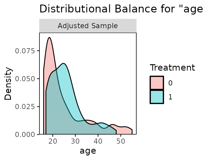
bal.plot(W.out, var.name = "race")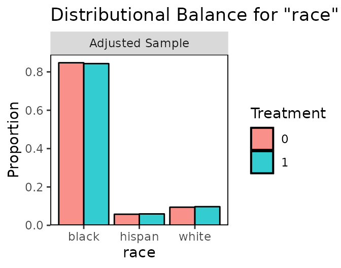
The first argument (or set of arguments) is the sufficient set of
arguments for a simple call to bal.tab(), defining the data
object (e.g., the output of a conditioning function), the treatment
indicators, and the weights or subclasses. See above for examples. The
next argument is the name of the covariate for which distributional
balance is to be assessed. If subclassification is used (i.e., if
subclasses are present in the input data object or arguments), an
additional argument which.sub can be specified, with a
number corresponding to the subclass number for which balance is to be
assessed on the specified covariate; if it is not specified, plots for
all subclasses will be displayed.
The user can also specify whether distributional balance is to be
shown before or after adjusting or both by using the argument to
which. If which = "unadjusted", balance will
be displayed for the unadjusted sample only. If
which = "both", balance will be displayed for both the
unadjusted sample and the adjusted sample. The default is to display
balance for the adjusted sample.
The output of bal.plot() is a density plot, histogram,
or empirical CDF plot for the two groups on the given covariate,
depending on the argument to type. For categorical or
binary variables, a bar graph is displayed instead. When multi-category
categorical variables are given, bars will be created for each level,
unlike in bal.tab(), which splits the variable into several
binary variables. The degree to which the densities for the two groups
overlap is a good measure of group balance on the given covariate;
significant differences in shape can be indicative of poor balance, even
when the mean differences and variance ratios are well within
thresholds. Strong distributional similarity is especially important for
variables strongly related to the outcome of interest.
Distributional balance can also be assessed on the distance measure,
and this can form an alternative to other common support checks, like
MatchIt’s plot(..., type = "hist") or
twang’s plot(..., plots = "boxplot"). To examine
the distributions of the distance measure, the input to
var.name must be the name of the distance variable. If the
data input object doesn’t already contain the distance measure (e.g., if
not using one of the conditioning packages), the distance measure must
be manually added as an input to bal.plot() through
distance, in addition to being called through
var.name.
Below is an example using bal.plot() to display the
distributions of propensity scores before and after weighting
adjustment:
#Before and after weighting; which = "both"
bal.plot(W.out, var.name = "prop.score",
         which = "both",
         type = "histogram",
         mirror = TRUE)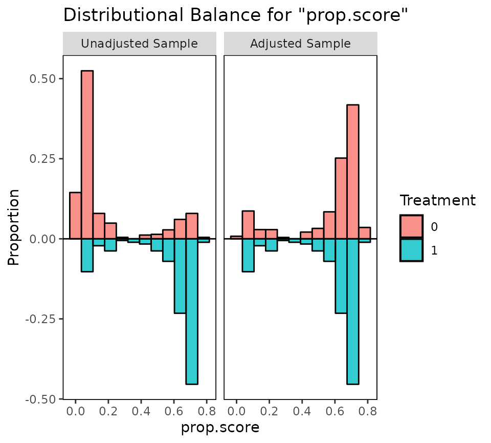
Setting type = "histogram" produces a histogram rather
than a density plot, and setting mirror = TRUE creates a
mirrored plot rather than overlapping histograms. Mirroring only works
with binary treatments.
It is generally not a useful assessment of balance to examine the overlap of the distance measure distributions after adjustment, as most conditioning methods will yield good distributional overlap on the distance measure whether or not balance is achieved on the covariates (Stuart et al. 2013). However, it may be useful to see the new range of the distance measure if calipers or common support pruning are used.
The output plot is made using ggplot2, which means that users familiar with ggplot2 can adjust the plot with ggplot2 commands.
When the treatment variable is continuous, users can use
bal.plot() to examine and assess dependence between the
covariate and treatment. The arguments given to bal.plot()
are the same as in the binary treatment case, but the resulting plots
are different. If the covariate is continuous, a scatterplot between the
covariate and the treatment variable will be displayed, along with a
linear fit line, a Loess curve, and a reference line indicating linear
independence. Used together, these lines can help diagnose departures
from independence beyond the simple correlation coefficient. Proximity
of the fit lines to the reference line is suggestive of independence
between the covariate and treatment variable. If the covariate is
categorical (including binary), density plots of the treatment variable
for each category will be displayed. Densities that overlap completely
are indicative of independence between the covariate and treatment. See
the section “Using cobalt with continuous treatments” for more details
and an example.
love.plot()
The Love plot is a summary plot of covariate balance before and after
conditioning popularized by Dr. Thomas E. Love. In a visually appealing
and clear way, balance can be presented to demonstrate to readers that
balance has been met within a threshold, and that balance has improved
after conditioning [which is not always the case; cf. King and Nielsen (2019)].
love.plot() does just this, providing the user with several
options to customize their plot for presentation. Below is an example of
its use:
data("lalonde", package = "cobalt")

# Nearest neighbor 1:1 matching with replacement
m.out <- MatchIt::matchit(treat ~ age + educ + married + race +
                              nodegree + re74 + re75,
                          data = lalonde,
                          method = "nearest",
                          replace = TRUE)

love.plot(m.out, binary = "std", thresholds = c(m = .1))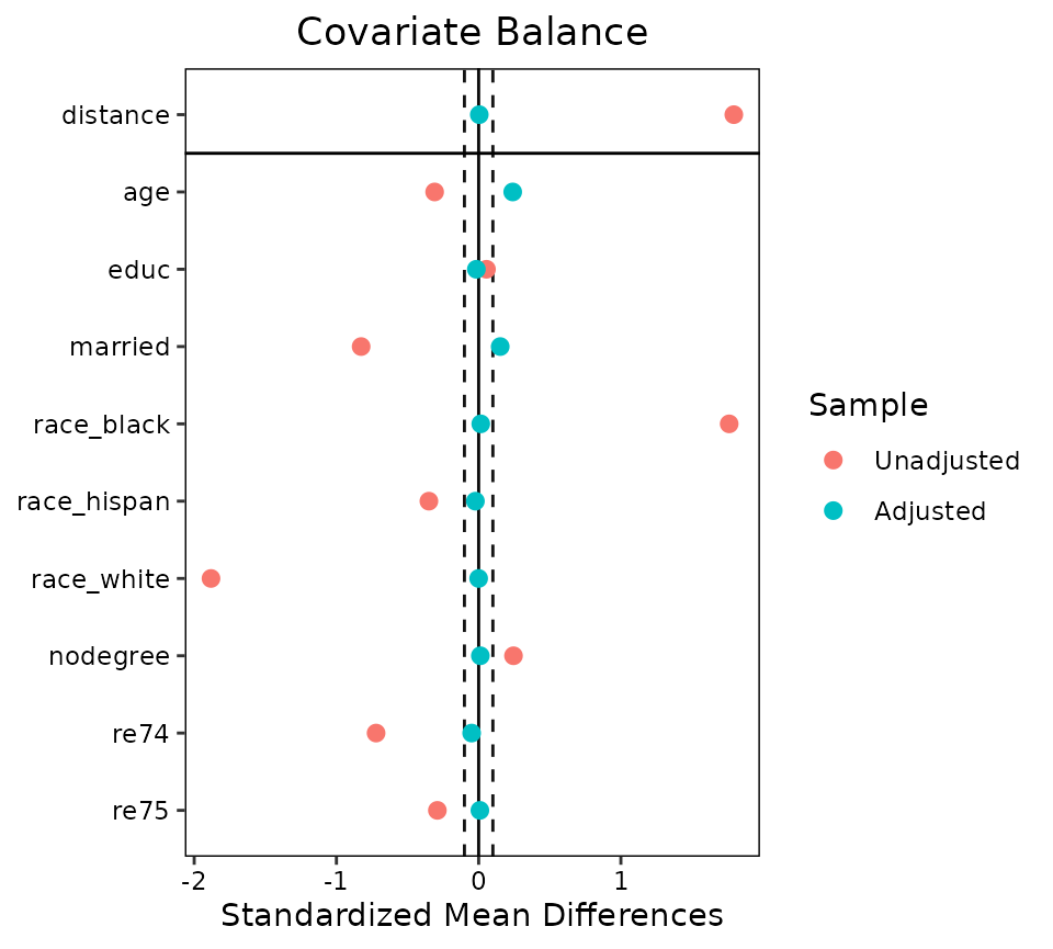
love.plot() takes as its arguments the same ones that
would go into a call to bal.tab(). In addition, it can take
as its first argument the output of a call to bal.tab();
this can be accomplished simply by inserting the bal.tab()
call into the first argument or by saving the result of a call to
bal.tab() to an object and inserting the object as the
argument. There are several other arguments, all of which control
display, that are described below.
The output is a plot with the balance statistic on the X-axis and the
covariates output in bal.tab() on the Y-axis. Each point
represents the balance statistic for that covariate, colored based on
whether it is calculated before or after adjustment. The dotted lines
represent the threshold set in the threshold argument; if
most or all of the points after adjustment are within the threshold,
that is good evidence that balance has been achieved.
The default is to present the absolute mean differences as they are
calculated in the call to bal.tab(); by specifying
stats = "variance.ratios" or
stats = "ks.statistics" (abbreviations allowed), the user
can request variance ratios or KS statistics instead or in addition.
Because binary variables don’t have variance ratios calculated, there
will not be rows for these variables, but these rows can be added (with
empty entries) to be in alignment with mean differences by setting
drop.missing = FALSE.
The thresholds argument works similarly to how it does
in bal.tab(); specifying it is optional, but doing so will
provide an additional point of reference on which to evaluate the
displayed balance measures.
If mean difference are requested, love.plot() will use
the mean differences as they are calculated by bal.tab()
and presented in the mean differences columns of the balance table. See
the section on using bal.tab() to see what the default
calculations are for these values. If abs = TRUE in
love.plot(), the plot will display absolute mean
differences, which can aid in display clarity since the magnitude is
generally the more important aspect of the statistic.
The order of the covariates displayed can be adjusted using the
argument to var.order. If left empty or NULL,
the covariates will be listed in the order of the original dataset. If
"adjusted", covariates will be ordered by the requested
balance statistic of the adjusted sample. If "unadjusted",
covariates will be ordered by the requested balance statistic of the
unadjusted sample, which tends to be more visually appealing.
Abbreviations are allowed. The distance variable(s), if any, will always
be displayed at the top. They can be omitted by setting
drop.distance = TRUE.
The plot uses the original variable names as they are given in the
data set, which may not be the names desired for display in publication.
By using the argument to var.names, users can specify their
own variable names to be used instead. To specify new variable names
with var.names, the user must enter an object containing
the new variable names and, optionally, the old variable names to
replace. For options of how to do so, see the help file for
love.plot() with ?love.plot. Below is an
example, creating a publication-ready plot with a few other arguments to
customize output:
v <- data.frame(old = c("age", "educ", "race_black", "race_hispan",
                        "race_white", "married", "nodegree", "re74", "re75", "distance"),
                new = c("Age", "Years of Education", "Black",
                        "Hispanic", "White", "Married", "No Degree Earned",
                        "Earnings 1974", "Earnings 1975", "Propensity Score"))

love.plot(m.out, stats = c("mean.diffs", "ks.statistics"),
          threshold = c(m = .1, ks = .05),
          binary = "std",
          abs = TRUE,
          var.order = "unadjusted",
          var.names = v,
          limits = c(0, 1),
          grid = FALSE,
          wrap = 20,
          sample.names = c("Unmatched", "Matched"),
          position = "top",
          shapes = c("circle", "triangle"),
          colors = c("red", "blue"))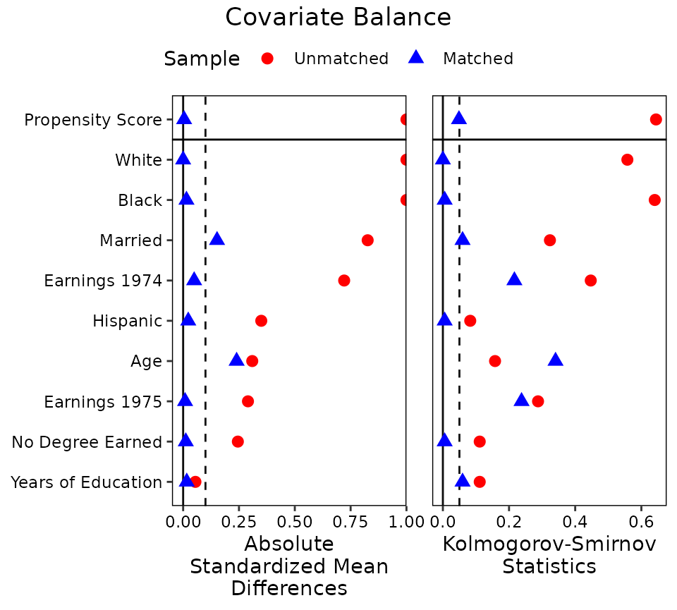
This plot shows that balance was improved on almost all variables after adjustment, bringing all but two below the threshold of .1 for absolute mean differences.
A helper function, var.names() can be used to more
easily create new variable names when many variables are present. See
?var.names for details.
When the treatment variable is continuous, love.plot()
will display Pearson correlations between each covariate and treatment.
The same arguments apply except that stats is ignored and
threshold corresponds to r.threshold, the
threshold for correlations.
Like the output of bal.plot(), the output of
love.plot() is a ggplot2 object, which means
ggplot2 users can modify the plot to some extent for
presentation or publication. Several aspects of the appearance of the
plot can be customized using the love.plot() syntax,
including the size, shape, and color of the points, the title of the
plot, whether to display grid lines, and whether to display lines
connecting the points. See ?love.plot for details. It may
be challenging to make adjustments to these aspects using
ggplot2 syntax, so these arguments allow for some simple
adjustments. See vignette("love.plot") for information on
more of love.plot()’s features.
Additional Features
Using cobalt with continuous treatments
Although the most common use of propensity scores is in the context of binary treatments, it is also possible to use propensity scores with continuous treatment to estimate dose-response functions while controlling for background variables (Hirano and Imbens 2005). As in the binary case, the goal of propensity score adjustment in the continuous case is to arrive at a scenario in which, conditional on the propensity score, treatment is independent of background covariates. When this is true (and there are no unmeasured confounders), treatment is also independent of potential outcomes, thereby meeting the strong ignorability requirement for causal inference.
Bia and Mattei (2008) describe the
use of the gpscore function in Stata, which appears to be
effective for estimating and assessing dose-response functions for
continuous treatments. In R, there are not many ways to estimate and
condition on the propensity score in these contexts. It is possible,
using the formulas described by Hirano and Imbens
(2005), to
generate the propensity scores manually and perform weighting,
subclassification, or covariate adjustment on them. The
WeightIt package supports continuous treatments with a variety
of options, including the CBPS method implemented in the CBPS
package and described by Fong et al. (2018), GBM
as described by Zhu et al. (2015), and
entropy balancing as described by Vegetabile et
al. (2021),
among others.
In cobalt, users can assess and present balance for
continuous treatments using bal.tab(),
bal.plot(), and love.plot(), just as with
binary treatments. The syntax is almost identical in both cases
regardless of the type of treatment variable considered, but there are a
few differences and specifics worth noting. The approach cobalt
takes to assessing balance is to display correlations between each
covariate and the treatment variable, which is the approach used in
CBPS and described in Zhu et al. (2015) and
Austin (2019), but
not that described in Hirano and Imbens (2005) or
implemented in gpscore (Bia and Mattei
2008), which involves stratifying on both the treatment
variable and the propensity score and calculating mean differences. Note
that the weighted correlations use the unweighted standard deviations of
the treatment variable and covariate in the denominator, so correlations
above 1 may be observed in rare cases. Correlations can be computed as
Pearson correlations, Spearman correlations (Pearson correlations on the
ranks), or distance correlations.
In addition to assessing the treatment-covariate correlations, it is important to assess the degree to which the adjusted sample is representative of the original target population. If the weighted sample differs greatly from the original sample, the estimated effect may be biased for the target population of interest, even if the covariates are independent from treatment. cobalt offers methods to compare the weighted sample to the unweighted sample in the context of continuous treatments, such as computing the standardized mean difference or KS statistic between the weighted and unweighted sample for each covariate.
Below is an example of the workflow for using propensity scores for
continuous treatments in the WeightIt package. To demonstrate,
we use the lalonde package included in cobalt,
using an arbitrary continuous variable as the treatment, though
substantively this analysis makes little sense.
data("lalonde", package = "cobalt")

#Generating weights with re75 as the continuous treatment
W.out.c <- WeightIt::weightit(re75 ~ age + educ + race + married +
                                  nodegree + re74,
                              data = lalonde,
                              method = "glm",
                              density = "kernel")
First, we can assess balance numerically using
bal.tab(). The default balance statistic used is the
Pearson correlation between each covariate and the treatment variable. A
threshold for balance on correlations can be specified using
thresholds; Zhu et al. (2015)
recommend using .1 as indicating balance, but in general lower is
better. Because the goal is complete independence between treatment and
covariates, not simply the absence of a linear correlation between
treatment and covariates, including interactions and polynomial terms
through the use of arguments to int and poly
is recommended (we just display the use of poly here for
brevity). Requesting the distance correlation can also be useful for
assessing independence because they are 0 only when the treatment and
covariate are completely independent, not just uncorrelated. In addition
to treatment-covariate correlations, we request KS statistics between
the weighted and unweighted samples by include "ks" (for
"ks.statistics.target") in the argument to
stats along with "c" (for
"correlations").
#Assessing balance numerically
bal.tab(W.out.c, stats = c("c", "k"), un = TRUE,
        thresholds = c(cor = .1), poly = 3)
## Balance Measures
## Type Corr.Un Corr.Adj R.Threshold KS.Target.Adj
## age Contin. 0.1400 -0.0342 Balanced, <0.1 0.1675
## educ Contin. 0.0183 0.0177 Balanced, <0.1 0.0573
## race_black Binary -0.1405 -0.0041 Balanced, <0.1 0.1036
## race_hispan Binary 0.0616 -0.0040 Balanced, <0.1 0.0138
## race_white Binary 0.0978 0.0067 Balanced, <0.1 0.0898
## married Binary 0.3541 -0.0435 Balanced, <0.1 0.2881
## nodegree Binary -0.0705 -0.0301 Balanced, <0.1 0.0022
## re74 Contin. 0.5520 -0.0676 Balanced, <0.1 0.3437
## age² Contin. 0.0998 -0.0449 Balanced, <0.1 0.1675
## educ² Contin. 0.0312 0.0264 Balanced, <0.1 0.0573
## re74² Contin. 0.4607 -0.1058 Not Balanced, >0.1 0.3437
## age³ Contin. 0.0627 -0.0538 Balanced, <0.1 0.1675
## educ³ Contin. 0.0361 0.0308 Balanced, <0.1 0.0573
## re74³ Contin. 0.3790 -0.1121 Not Balanced, >0.1 0.3437
##
## Balance tally for treatment correlations
## count
## Balanced, <0.1 12
## Not Balanced, >0.1 2
##
## Variable with the greatest treatment correlation
## Variable Corr.Adj R.Threshold
## re74³ -0.1121 Not Balanced, >0.1
##
## Effective sample sizes
## Total
## Unadjusted 614.
## Adjusted 55.55We can also visually assess balance using bal.plot().
For continuous covariates, bal.plot() displays a
scatterplot of treatment against the covariate, and includes a linear
fit line (red), a smoothed fit curve (blue), and a horizontal reference
line (black) at the unweighted mean of the treatment variable, and a
vertical line at the unweighted mean of the covariate. These lines can
be used to diagnose dependence. If either fit line is not close to flat
and not lying on top of the reference line, there may be some remaining
dependence between treatment and the covariate. The points in the
weighted plot are shaded according to the size of their corresponding
weight. If the linear fit line (red) does not cross through the
intersection of the black reference lines, the target population of the
weighted estimate differs from the original population. For categorical
covariates, including binary, bal.plot() displays a density
plot of the treatment variable in each category. If treatment and the
covariate are independent, the densities for each category should
overlap with each other. A distinct lack of overlap is indicative of
remaining dependence between treatment and the covariate.
#Assessing balance graphically
bal.plot(W.out.c, "re74", which = "both")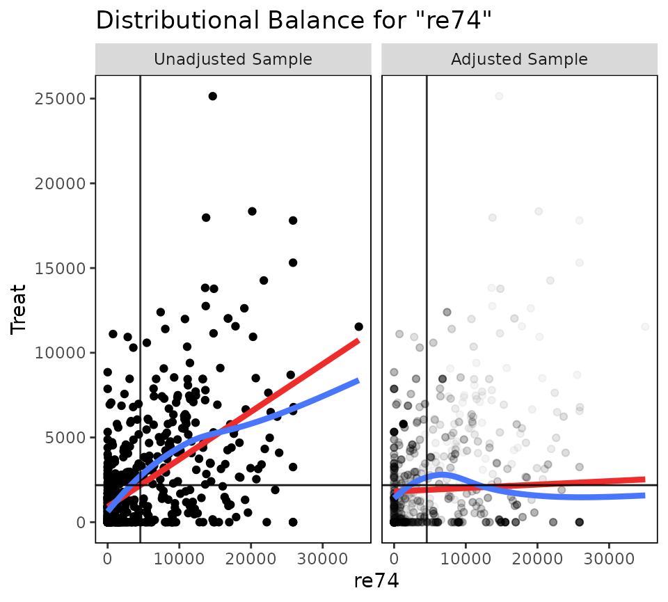
bal.plot(W.out.c, "married", which = "both")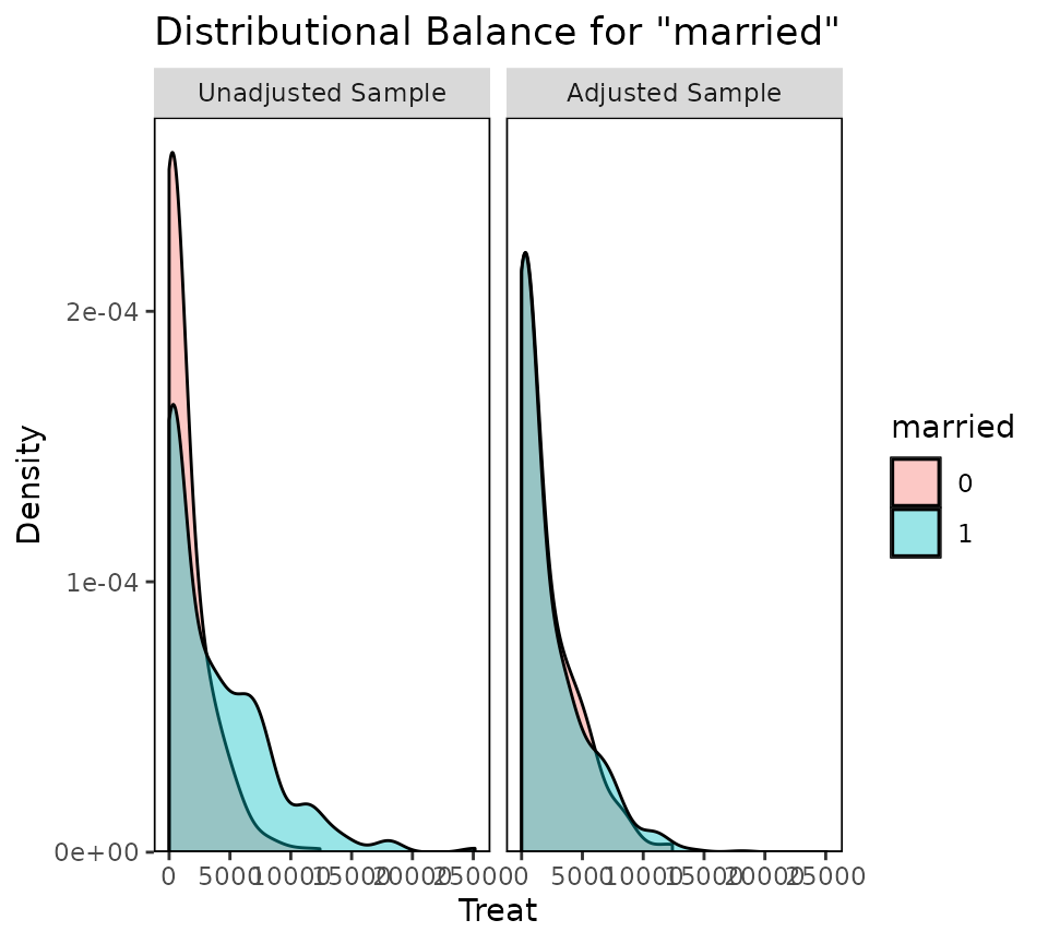
When balance has been achieved to a satisfactory level, users can
present balance improvements in a Love plot using the
love.plot() command, just as with binary treatments.
#Summarizing balance in a Love plot
love.plot(W.out.c, stats = c("c", "ks"),
          thresholds = c(cor = .1),
          abs = TRUE, wrap = 20,
          limits = list(ks = c(0, .5)),
          var.order = "unadjusted", line = TRUE)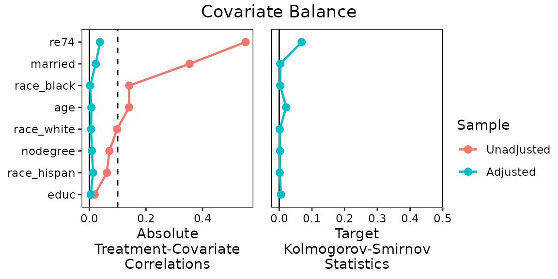
Using cobalt with multi-category treatments
When multiple categorical treatment groups are to be compared with each other, it is possible to create balance across the treatment groups using preprocessing methods. Lopez and Gutman (2017) compare methods used to create balance with multi-category treatments and briefly describe balance assessment for these scenarios. An important note is the choice of estimand to be examined. The ATE represents the causal effect of moving from one treatment group to another for all units in the population; the ATT represents the causal effect of moving from one treatment group to another “focal” treatment group for just the units that would have been in the focal treatment group. The way balance is assessed in these scenarios differs. For the ATE, all possible treatment pairs must be assessed for balance because all possible comparisons are potentially meaningful, but for the ATT, only treatment pairs that include the focal treatment group can be meaningfully compared, so balance needs only to be assessed in these pairs.
In cobalt, users can assess and present balance for
multi-category treatments using bal.tab(),
bal.plot(), and love.plot(), just as with
binary treatments. The output is slightly different, though, and is
similar to the output generated when using these functions with
clusters. bal.tab() computes balance statistics for all
pairwise comparisons between treatment groups and a table containing the
worst balance for each covariate across pairwise comparisons. For mean
differences, this is described in Lopez and
Gutman (2017)
as “Max2SB,” or the maximum pairwise standardized bias. In
cobalt, this has been extended to variance ratios and KS
statistics as well. If the worst imbalance is not too great, then
imbalance for all pairwise comparisons will not be too great either.
When the ATT is desired, a focal group must be specified (unless done so
automatically for some methods), and only the treatment group
comparisons that involve that focal group will be computed and
displayed.
love.plot() allows for the display of each pairwise
treatment or the range of balance across treatment pairs for each
covariate. bal.plot() displays distributional balance for
the requested covariate across all treatment groups.
Below is an example of using cobalt with multi-category
treatments. For this example, race will be the “treatment”;
this type of analysis is not meant to be causal, but rather represents a
method to examine disparities among groups accounting for covariates
that might otherwise explain differences among groups. We will use
WeightIt to generate balanced groups by estimating generalized
propensity score weights using multinomial logistic regression.
data("lalonde", package = "cobalt")

#Using WeightIt to generate weights with multinomial
#logistic regression
W.out.mn <- WeightIt::weightit(race ~ age + educ + married +
                                   nodegree + re74 + re75,
                               data = lalonde,
                               method = "glm")
First, we can examine balance numerically using
bal.tab(). There are three possible pairwise comparisons,
all of which can be requested with which.treat = .all. See
?bal.tab.multi for more details.
#Balance summary across treatment pairs
bal.tab(W.out.mn, un = TRUE)
## Balance summary across all treatment pairs
## Type Max.Diff.Un Max.Diff.Adj
## age Contin. 0.3065 0.0557
## educ Contin. 0.5861 0.1140
## married Binary 0.3430 0.0297
## nodegree Binary 0.2187 0.0546
## re74 Contin. 0.6196 0.1527
## re75 Contin. 0.3442 0.1491
##
## Effective sample sizes
## black hispan white
## Unadjusted 243. 72. 299.
## Adjusted 138.38 54.99 259.59
#Assessing balance for each pair of treatments
bal.tab(W.out.mn, un = TRUE,
        disp = "means",
        which.treat = .all)
## Balance by treatment pair
##
## - - - black (0) vs. hispan (1) - - -
## Balance Measures
## Type M.0.Un M.1.Un Diff.Un M.0.Adj M.1.Adj Diff.Adj
## age Contin. 26.0123 25.9167 -0.0101 26.6155 27.0006 0.0408
## educ Contin. 10.2346 9.0139 -0.4515 10.5033 10.1950 -0.1140
## married Binary 0.2222 0.4444 0.2222 0.4109 0.3840 -0.0269
## nodegree Binary 0.6955 0.7639 0.0684 0.6005 0.6552 0.0546
## re74 Contin. 2499.4492 4431.6260 0.3183 5486.7968 4740.5305 -0.1229
## re75 Contin. 1613.7752 2741.3920 0.3442 2665.9699 2229.2822 -0.1333
##
## Effective sample sizes
## black hispan
## Unadjusted 243. 72.
## Adjusted 138.38 54.99
##
## - - - black (0) vs. white (1) - - -
## Balance Measures
## Type M.0.Un M.1.Un Diff.Un M.0.Adj M.1.Adj Diff.Adj
## age Contin. 26.0123 28.8094 0.2963 26.6155 27.1412 0.0557
## educ Contin. 10.2346 10.5987 0.1347 10.5033 10.3204 -0.0676
## married Binary 0.2222 0.5652 0.3430 0.4109 0.4137 0.0028
## nodegree Binary 0.6955 0.5452 -0.1503 0.6005 0.6246 0.0240
## re74 Contin. 2499.4492 6260.5029 0.6196 5486.7968 4560.0208 -0.1527
## re75 Contin. 1613.7752 2515.1320 0.2752 2665.9699 2177.6625 -0.1491
##
## Effective sample sizes
## black white
## Unadjusted 243. 299.
## Adjusted 138.38 259.59
##
## - - - hispan (0) vs. white (1) - - -
## Balance Measures
## Type M.0.Un M.1.Un Diff.Un M.0.Adj M.1.Adj Diff.Adj
## age Contin. 25.9167 28.8094 0.3065 27.0006 27.1412 0.0149
## educ Contin. 9.0139 10.5987 0.5861 10.1950 10.3204 0.0464
## married Binary 0.4444 0.5652 0.1208 0.3840 0.4137 0.0297
## nodegree Binary 0.7639 0.5452 -0.2187 0.6552 0.6246 -0.0306
## re74 Contin. 4431.6260 6260.5029 0.3013 4740.5305 4560.0208 -0.0297
## re75 Contin. 2741.3920 2515.1320 -0.0691 2229.2822 2177.6625 -0.0158
##
## Effective sample sizes
## hispan white
## Unadjusted 72. 299.
## Adjusted 54.99 259.59
## - - - - - - - - - - - - - - - - - - - - - - - -We can also assess balance graphically. The same guidelines apply for multi-category treatments as do for binary treatments. Ideally, covariate distributions will look similar across all treatment groups.
#Assessing balance graphically
bal.plot(W.out.mn, "age", which = "both")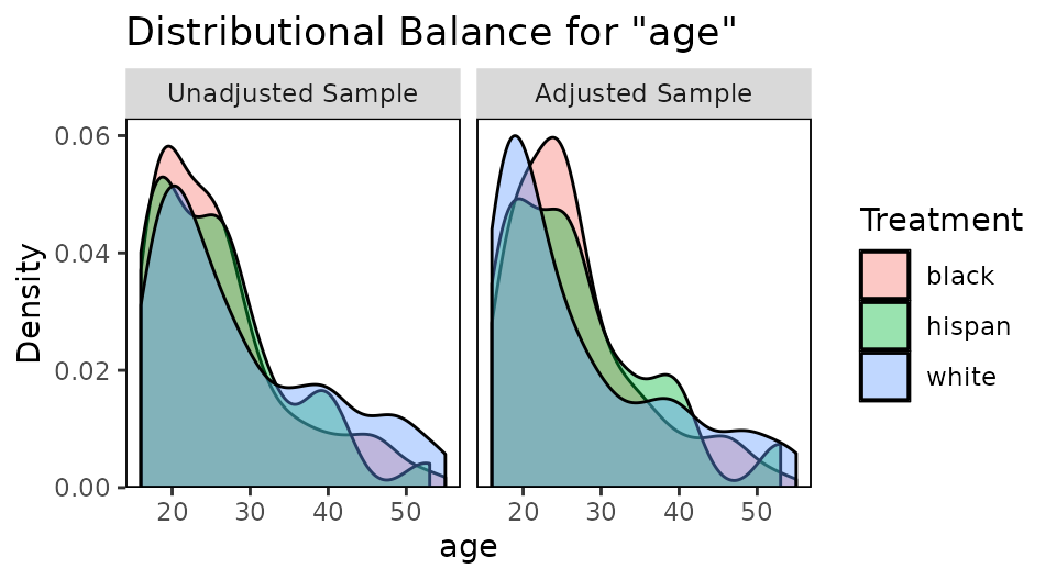
bal.plot(W.out.mn, "married", which = "both")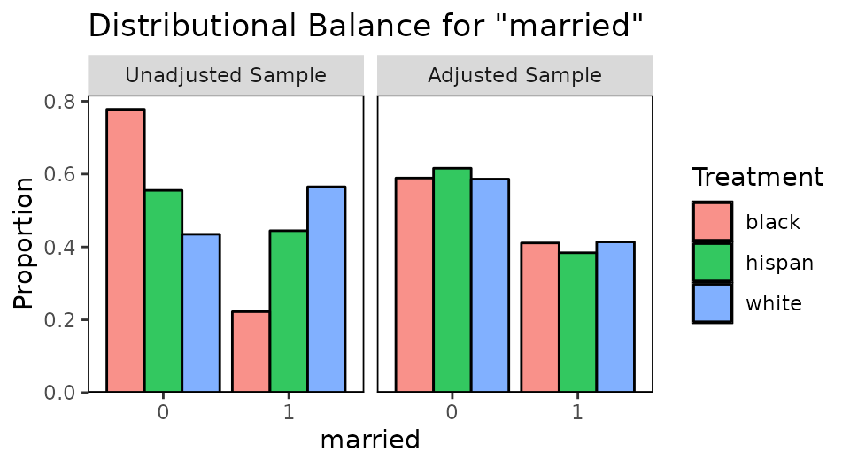
Finally, we can use love.plot() to display balance
across treatments. By default, love.plot() displays the
values in the summary across pairwise comparisons. To request individual
treatment comparisons, use which.treat = .all in
love.plot().
#Summarizing balance in a Love plot
love.plot(W.out.mn, thresholds = c(m = .1), binary = "std",
          which.treat = .all, abs = FALSE)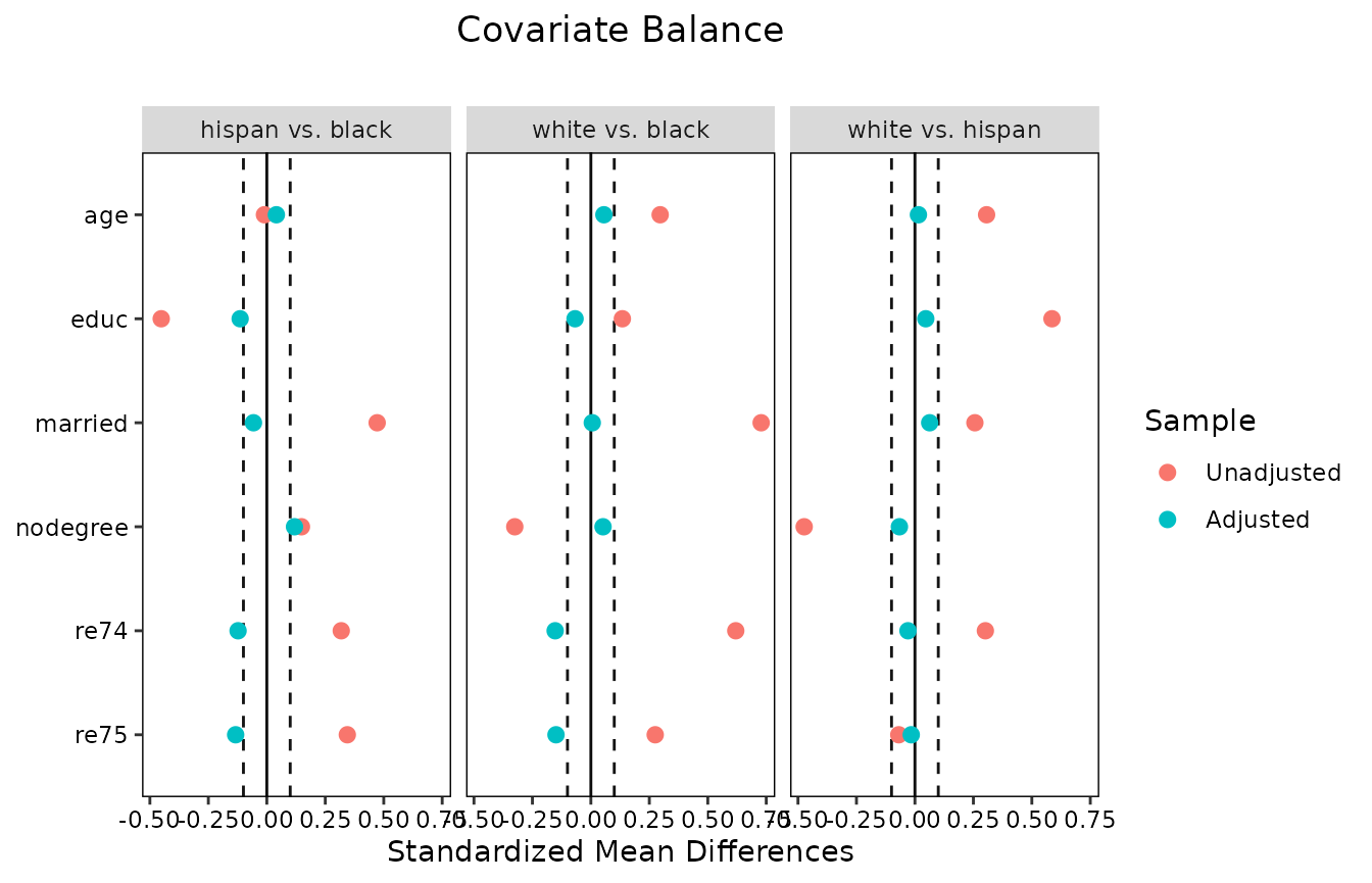
Comparing balancing methods
It is possible to display balance for multiple balancing methods at
the same time in bal.tab(), bal.plot(), and
love.plot(). To do so, weights generated from each
balancing method need to be supplied together in each call. This can be
done by supplying the weights or the output objects themselves. For
example, we can compare matching and inverse probability weighting for
the ATT using the following code and the output generated above.
bal.tab(treat ~ age + educ + married + race +
            nodegree + re74 + re75, data = lalonde,
        weights = list(Matched = m.out,
                       IPW = W.out),
        disp.v.ratio = TRUE)
## Balance Measures
## Type Diff.Matched V.Ratio.Matched Diff.IPW V.Ratio.IPW
## age Contin. 0.2395 0.5565 0.1112 0.5086
## educ Contin. -0.0161 0.5773 -0.0641 0.6018
## married Binary 0.0595 . -0.0938 .
## race_black Binary 0.0054 . -0.0044 .
## race_hispan Binary -0.0054 . 0.0016 .
## race_white Binary 0.0000 . 0.0028 .
## nodegree Binary 0.0054 . 0.1151 .
## re74 Contin. -0.0493 1.0363 -0.0039 1.4821
## re75 Contin. 0.0087 2.1294 -0.0428 1.1712
##
## Effective sample sizes
## Control Treated
## All 429. 185
## Matched 46.31 185
## IPW 108.2 185To use bal.plot(), the same syntax can be used:
bal.plot(treat ~ age, data = lalonde,
         weights = list(Matched = m.out,
                        IPW = W.out),
         var.name = "age", which = "both")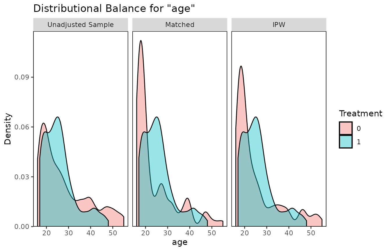
With love.plot(), var.order can be
"unadjusted", "alphabetical", or one of the
names of the weights to order the variables. Also, colors
and shapes should have the same length as the number of
weights or have length 1.
love.plot(treat ~ age + educ + married + race +
              nodegree + re74 + re75,
          data = lalonde,
          weights = list(Matched = m.out,
                         IPW = W.out),
          var.order = "unadjusted", binary = "std",
          abs = TRUE, colors = c("red", "blue", "darkgreen"),
          shapes = c("circle", "square", "triangle"),
          line = TRUE)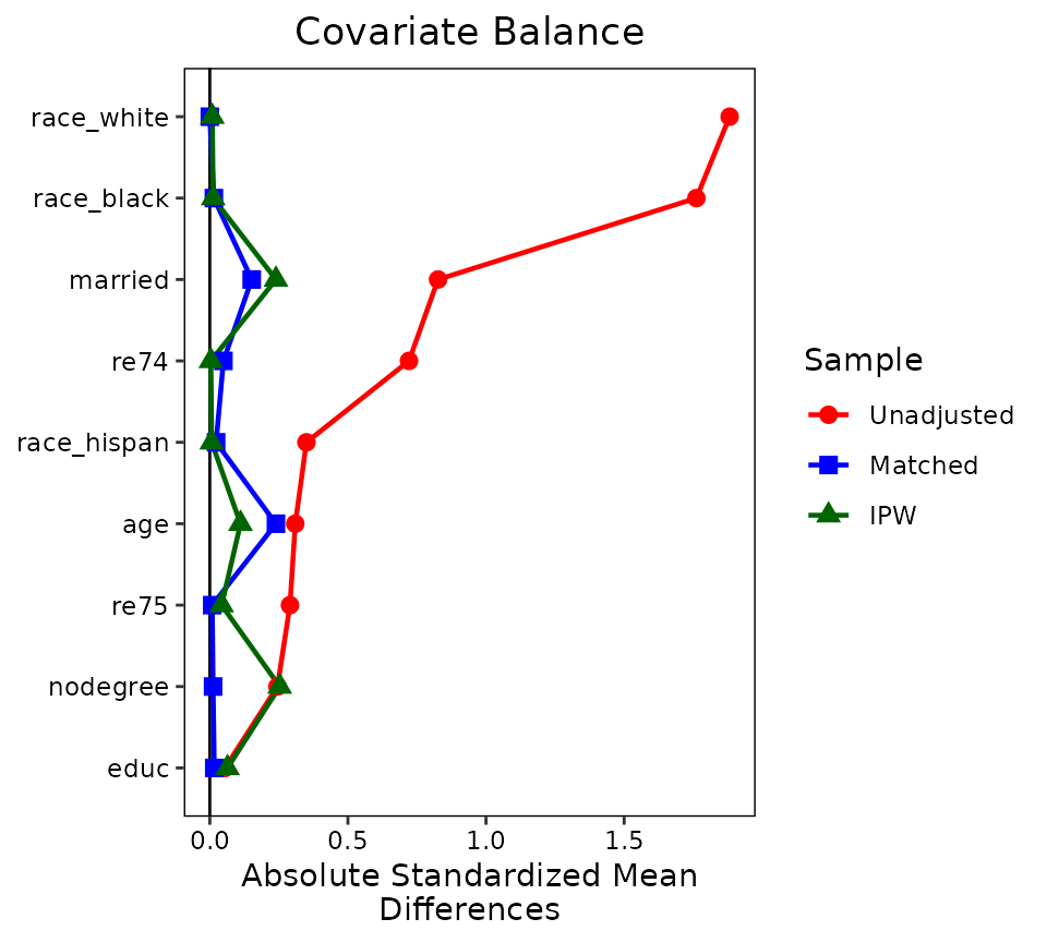
Another way to compare weights from multiple objects is to call
bal.tab() with one object as usual and supply the other(s)
to the weights argument; see below for an example:
Using the prognostic score for balance assessment
The prognostic score is the model-predicted outcome for an individual, excluding the treatment variable in the model (Hansen 2008). Stuart et al. (2013) found that prognostic scores can be an extremely effective tool for assessing balance, greatly outperforming mean differences on covariates and significance tests. This is true even if the prognostic score model is slightly misspecified. Although the use of prognostic scores appears to violate the spirit of preprocessing in that users observe the outcome variable prior to treatment effect estimation, typically the prognostic score model is estimated in just the control group, so that the outcome of the treated group (which may contain treatment effect information) is excluded from analysis.
Assessing balance on the prognostic score is simple in cobalt, and highly recommended when available. The steps are:
- Estimate the outcome model in the control group
- Generate model-predicted outcome values for both the treated and control groups
- Assess balance on prognostic scores by comparing standardized mean differences
To use prognostic scores in cobalt, simply add the
prognostic score as a variable in the argument to distance.
Below is an example of how to do so after a call to
matchit():
ctrl.fit <- glm(re78 ~ age + educ + race +
                    married + nodegree + re74 + re75,
                data = lalonde,
                subset = treat == 0)
lalonde$prog.score <- predict(ctrl.fit, newdata = lalonde)

bal.tab(m.out, stats = c("m", "ks"),
        distance = lalonde["prog.score"])
## Balance Measures
## Type Diff.Adj KS.Adj
## prog.score Distance -0.0485 0.1351
## distance Distance 0.0044 0.0486
## age Contin. 0.2395 0.3405
## educ Contin. -0.0161 0.0595
## married Binary 0.0595 0.0595
## race_black Binary 0.0054 0.0054
## race_hispan Binary -0.0054 0.0054
## race_white Binary 0.0000 0.0000
## nodegree Binary 0.0054 0.0054
## re74 Contin. -0.0493 0.2162
## re75 Contin. 0.0087 0.2378
##
## Sample sizes
## Control Treated
## All 429. 185
## Matched (ESS) 46.31 185
## Matched (Unweighted) 82. 185
## Unmatched 347. 0
bal.plot(m.out, "prog.score",
         distance = lalonde["prog.score"],
         which = "both")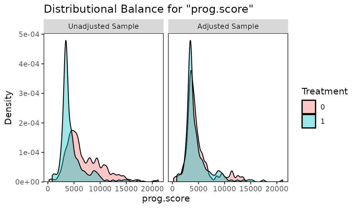
Although the prognostic score is sensitive to the outcome estimation
model used, a defensible prognostic score model can yield valid
prognostic scores, which can then be used in balance assessment. In the
above example, balance on the estimated prognostic score was good, so we
can have some confidence that the effect estimate will be relatively
unbiased, even though the age variable remains imbalanced.
The logic is that that age is not a highly prognostic variable, which
could be demonstrated by examining the standardized regression output of
prognostic score model, so even though imbalance remains, such imbalance
is unlikely to affect the effect estimate. The variables
re74 and re75, though, which are highly
prognostic of the outcome, are quite balanced, thereby supporting an
unbiased treatment effect estimate.
Details on Calculations
There are calculations in cobalt that may be opaque to
users; this section explains them. For even more details, see
vignette("faq").
Variance in Standardized Mean Differences and Correlations
When computing a standardized mean difference, the raw mean
difference is divided by a standard deviation, yielding a d-type effect
size statistic. In bal.tab(), the user can control whether
the standard deviation is that of the treated group or control group or
a pooled estimate, calculated as the square root of the average of the
group variances. In most applications, the standard deviation
corresponding to the default for the method is the most appropriate.
A key detail is that the standard deviation, no matter how it is computed, is always computed using the unadjusted sample4. This is line with how MatchIt computes standardized mean differences5, and is recommended by Stuart (2008, 2010). One reason to favor the use of the standard deviation of the unadjusted sample is that it prevents the paradoxical situation that occurs when adjustment decreases both the mean difference and the spread of the sample, yielding a larger standardized mean difference than that prior to adjustment, even though the adjusted groups are now more similar. By using the same standard deviation before and after adjusting, the change in balance is isolated to the change in mean difference, rather than being conflated with an accompanying change in spread.
The same logic applies to computing the standard deviations that appear in the denominator of the treatment-covariate correlations that are used to assess balance with continuous treatments. Given that the covariance is the relevant quality to be assessed and the correlation is just a standardization used to simplify interpretation, the standardization factor should remain the same before and after adjustment. Thus, the standard deviations of the unadjusted sample are used in the denominator of the treatment-covariate correlation, even when the correlation in question is for the adjusted sample.
Note that when sampling weights are used, values for the unadjusted sample will be computed incorporating the sampling weights; in that sense, they are “adjusted” by the sampling weights.
Weighted Variance
When using weighting or matching, summary values after adjustment are calculated by using weights generated from the matching or weighting process. For example, group means are computed using the standard formula for a weighted mean, incorporating the weighting or matching weights into the calculation. To estimate a weighted sample variance for use in variance ratios, sample standard deviations, or other statistics in the presence of sampling weights, there are two formulas that have been proposed:
\(\frac{\sum_{i=1}^{n} w_{i}(x_{i} - \bar{x}_{w})^2}{(\sum_{i=1}^{n} w_{i}) - 1}\)
\(\frac{\sum_{i=1}^{n} w_{i}}{(\sum_{i=1}^{n} w_{i})^2 - \sum_{i=1}^{n} w^2_{i}} \sum_{i=1}^{n} w_{i}(x_{i} - \bar{x}_{w})^2\)
The weights used in the first formula are often called “frequency weights”, while the weights in the second formula are often called normalized or “reliability weights”. MatchIt, twang, and Matching all use the first formula when calculating any weighted variance (CBPS does not compute a weighted variance). However, Austin (2008b) and Austin and Stuart (2015) recommend the second formula when considering matching weights for k:1 matching or weights for propensity score weighting. In cobalt, as of version 2.0.0, the second formula is used to remain in line with recommended practice. For some applications (e.g., when all weights are either 0 or 1, as in 1:1 matching), the two formulas yield the same variance estimate. In other cases, the estimates are nearly the same. For binary variables, the weighted variance is computed as \(\bar{x}_{w}(1-\bar{x}_{w})\) where \(\bar{x}_{w}\) is the weighted proportion of 1s in the sample.
Effective Sample Size for Weighting
Knowledge of the sample size after adjustment is important not just for outcome analysis but also for assessing the adequacy of a conditioning specification. For example, pruning many units through common support cutoffs, caliper matching, or matching with replacement can yield very small sample sizes that hurt both the precision of the outcome estimate and the external validity of the conclusion. In both matching and weighting, the adjusted sample size is not so straightforward because the purpose of weighting is to down- and up-weight observations to create two similar samples. The “effective sample size” (ESS) is a measure of the sample size a non-weighted sample would have to have to achieve the same level of precision as the weighted sample (Ridgeway 2006). This measure is implemented in twang using the following formula: \[ESS = \frac{(\sum_{i=1}^{n} w_{i})^2}{\sum_{i=1}^{n} w_{i}^2}\] Shook-Sa and Hudgens (2020) derived the specific relationship between the ESS and the standard error of a propensity score-weighted mean.
What’s Missing in cobalt
A fair amount is missing in cobalt that is present in other packages. Though there is value in many of the aspects that cobalt lacks, many were purposefully excluded based on methodological recommendations that conflict with the current use of some other packages. Below are aspects that are intentionally missing from cobalt that users may be used to from other packages. Their reasons for exclusion are included, with the hope that users of cobalt will be satisfied with what is available and be confident they are using the most methodologically sound tools for balance assessment.
Test Statistics and P-values
Some of the early literature on propensity score matching included measures for balance assessment that relied on hypothesis tests for the independence of treatment assignment and covariates after adjustment (e.g., Hansen 2004; Rosenbaum and Rubin 1985). In a review of propensity score applications in the social sciences, Thoemmes and Kim (2011) found that over 66% of studies used significance tests to assess balance. Likewise, Austin (2008a) found that over 70% of studies using propensity scores in the medical literature used significance tests to assess balance, a finding replicated by Ali et al. (2015). These hypothesis tests can come in many forms: t-tests for the difference in means between groups, chi-square tests for the difference in proportion between groups, Kolmogorov-Smirnov tests for the difference in cumulative density between groups, or F-tests for the difference in means between groups across subclasses.
The use of hypothesis tests appears natural here: if balance is achieved, we would not expect extreme values for the test statistics, and we can quantify the probability of observing imbalance as extreme as the one observed if no imbalance is present as a way to assess whether there is balance, as we can do with standard hypothesis testing. But this view is not shared by the methodological community: many contemporary propensity score methodologists recommend against using hypothesis tests for balance assessment (e.g., Ho et al. 2007; Imai et al. 2008; Austin 2011, 2009; Stuart 2010; Thoemmes and Kim 2011; Ali et al. 2015). There are logical reasons for this preference against hypothesis tests, noted clearly in Ali et al. (2015) and Linden (2014): they are influenced by sample size, which fluctuates during adjustment, and the theory behind them is inappropriate because balance is a quality solely of the sample in question, not in relation to a population. The relevant information in a hypothesis test for group differences is the standardized magnitude of the group difference, and so such a measure is preferred.
Because hypothesis tests can be misleading and their use is discouraged by leading methodologists, they have been completely excluded in cobalt in favor of summary statistics. This stands in contrast to twang, Matching, and RItools, all of which report hypothesis test p-values in their balance output.
Q-Q Plots and Summaries
Q-Q plots have been recommended as tools to assess distributional
balance of covariates between groups (Ho et al.
2007), and are implemented in MatchIt and
Matching (twang implements them but for a different
purpose). Statistics summarizing the degree of imbalance in Q-Q plots
are also reported in both MatchIt and Matching.
MatchIt’s summary() command reports “eQQ Mean” and
“eQQ Max” for each covariate before and after adjustment. These are the
mean and maximum distance between the treated and control group
empirical Q-Q plots on the scale of the covariate. Values close to 0
indicate good balance between groups for the given covariate.
A weakness of empirical Q-Q plots is that they don’t reveal much about the differences in the shapes of the distributions between the groups, which is a key aspect of distributional balance. A density plot essentially contains the same information, but is clearer and more intuitive. Although the assessment of balance using an empirical Q-Q plot is straightforward (i.e., deviations from the 45-degree line indicate imbalances), density plots present the information in a way more in line with the actual goals of conditioning, in particular, that the distributions of treated and control units are similar (Ho et al. 2007). Empirical Q-Q plot summary statistics may be useful in quantifying imbalance, but currently there are few recommendations for their use.
What’s Added in cobalt
There are several features in cobalt that are present in few, if any, balance assessment tools in the major packages. These come from methodological recommendations and requests by members of the methodological community.
Density Plots
As mentioned above, cobalt displays density plots and bar charts rather than empirical Q-Q plots for the assessment of distributional similarity. These charts are not standard in any of the conditioning packages, but can be an intuitive and helpful tool for deciding whether adjustment has yielded similar distributions between the groups for given covariates. Though there are no obvious heuristics for deciding how much dissimilarity is too much dissimilarity, density plots do avoid the sometimes confusing logic of empirical Q-Q plots in favor of simplicity and interpretability. Austin (2009) and Linden (2014) consider density plots as a compliment to empirical Q-Q plots to more finely examine balance after adjusting.
Variance Ratios
Although mean differences (including t-tests and chi-square tests)
are the most reported balance statistic (Thoemmes and Kim
2011), variance ratios have been recommended in the
literature as a means to further examine balance between groups (Austin 2009; Ho et al. 2007;
Imai
et al. 2008). When group variances are similar, the variance
ratio will be close to 1. Common thresholds for the variance ratio for
balanced groups are .5 and 2 (Stuart 2010; Rubin 2001),
though ratios closer to 1 are preferred. Although bal.tab()
in cobalt does not display variance ratios by default, they can
be easily requested and have thresholds set.
Distinguishing Continuous and Binary Covariates
Continuous and binary covariates are treated differently by default
in bal.tab() and bal.plot(). For continuous
covariates, the standard summaries apply: standardized mean differences,
variance ratios, and density plots. For binary covariates, raw
differences in proportion and bar charts are preferable, and variance
ratios are useless.
The value of standardized mean differences for continuous variables is that they are on the same scale so that they can be compared across variables, and they allow for a simple interpretation even when the details of the variable’s original scale are unclear to the analyst. None of these advantages are passed to binary variables because binary variables are already on the same scale (i.e., a proportion), and the scale is easily interpretable. In addition, the details of standardizing the proportion difference of a binary variable involve dividing the proportion difference by a variance, but the variance of a binary variable is a function of its proportion (Austin 2009). Standardizing the proportion difference of a binary variable can yield the following counterintuitive result: if \(X_{T} = .2\) and \(X_{C} = .3\), the standardized difference in proportion would be different from that if \(X_{T} = .5\) and \(X_{C} = .6\), even though the expectation is that the balance statistic should be the same for both scenarios because both would yield the same degree of bias in the effect estimate. In addition, Ali et al. (2014) found that the raw difference in proportion was a better predictor of bias than the standardized mean difference for binary variables6.
MatchIt allows users to view either standardized mean differences for all covariates or raw differences for all covariates, and twang and Matching display standardized differences for all variables but calculate test statistics depending on whether the covariate is continuous or binary (CBPS does not calculate mean differences, but presents both standardized and unstandardized means for all covariates). cobalt allows the user to select how the differences are to be calculated separately for continuous and binary variables, and uses the intuitive default that mean differences for continuous variables should be standardized while proportion differences for binary variables should not be.
Because the variance of a binary variable is a function only of its proportion, the variance ratio of a binary variable in two groups is a function only of their proportions, thereby containing no more information than the simple difference in proportion. Therefore, for binary variables, cobalt does not compute variance ratios, as they can be misleading.
Interactions and Polynomials
Because the goal of a balancing procedure is to achieve independence
between treatment and the joint distribution of covariates, evaluating
univariate distributional similarity may not be sufficient for assessing
balance completely. Some writers have recommended the evaluation of
distributional similarity of interaction and polynomial terms to account
for this. Rather than requiring the user to create interaction variables
by hand, bal.tab() can produce balance statistics for
interactions by specifying int = TRUE, similar to
MatchIt’s summary(), and polynomials by specifying
a numeric argument to poly (e.g., 2 for squared terms).
When including categorical variables in balance assessment,
bal.tab() makes a few adjustments under the hood that
deserve explanation. First, if a variable is binary and is entered as a
factor variable, balance statistics will only be displayed for one level
of the variable (since the other is redundant), but balance on
interaction terms will be displayed for all values of the variables.
For example, consider a binary variable “Sex” with values “Male” and
“Female”. Many functions, including bal.tab(),
lm(), and matchit(), will split this variable
into two numeric dummy variables, “Male” and “Female”, each of which
take on the values 0 and 1. One of these new variables is completely
redundant: all of the relevant information is stored in just “Female”,
so “Male” can be eliminated. Consider now a variable “Age”: what is
desired in balance assessment is the interaction between Age and Sex;
distributional similarity on the interaction between the treated and
untreated groups is evidence of multivariate balance. Computing the
interaction between “Female” and “Age” yields a variable that is “Age”
when the unit is female and 0 otherwise. The average value of this
variable is the average age of females in the sample, weighted by the
proportion of females. If the two treatment groups have similar average
values of this variable, this is taken as evidence for balance on the
interaction between sex and age, though it is entirely possible that the
average age of men differs greatly between the two groups. Thus, an
additional variable computed as the product of “Male” and “Age” would be
necessary to fully assess balance on the interaction between sex and
age. bal.tab() produces this interaction term, which would
otherwise be unobserved by the analyst7. The interactions
among levels of a single factor, which always be equal to 0, are
excluded in bal.tab().
Interactions between the distance measure and other variables have
been excluded in bal.tab(), noting that balance on the
distance measure is neither necessary nor sufficient for covariate
balance.
Because the number of computations increases both with sample size
and number of variables, computing interactions can be slow. In addition
to taking the product of variables two at a time, bal.tab()
checks variables to ensure no variables were created that contain only a
single value (e.g., interactions between mutually exclusive covariates)
or are redundant with respect to other variables (e.g., manually created
interactions or manually split factors). This results in cleaner, more
useful output, but also requires more computing time. It is advisable to
store the results of a call to bal.tab() to a variable to
be accessed later rather than to call bal.tab() several
times when using it with interactions.
Clusters
The use of preprocessing techniques in the context of multilevel data
(e.g., students within schools, patients within hospitals) has been
increasing. Currently no other package allows for any balance assessment
with respect to clusters, except by manually examining balance on
clusters specified manually. It can be useful to examine balance within
each cluster, but, especially if there are many clusters, it may also be
useful to examine a summary of balance across clusters. In all of its
functions, cobalt provides options for displaying balance on
clustered data sets. This can occur either within specified clusters or
across all clusters. Details on using cobalt with clustered
data can be found in vignette("segmented-data").
Missing Data
Missing data is frequent in all research involving human subjects,
and especially in the large survey data sets that are often used to
answer causal questions in the social sciences. cobalt
functions can assess balance not only on the observed covariates but
also on the proportion of missing values for each covariate.
Additionally, cobalt has features designed especially for
assessing balance on preprocessed data sets that have been multiply
imputed to address covariate missingness. Although the guidelines on
assessing balance on multiply imputed data sets are scarce, it is
valuable to assess balance within and across imputed data sets to ensure
the preprocessing solution is applicable to all imputations. Details on
using cobalt with multiply imputed data can be found in
vignette("segmented-data").
For Programmers: Integrating cobalt with Your Package
If you are designing a new R package for preprocessing that performs
similar functions to MatchIt, twang,
Matching, optmatch, CBPS, ebal,
designmatch, cem, or WeightIt, you might
consider integrating cobalt into your package to avoid
programming your own balance assessment tool. The simplest way to do so
is to have the output of your preprocessing function contain sufficient
elements for use with the default method for bal.tab() and
bal.plot(). See ?bal.tab.default for more
information on how this might work.
As cobalt is updated to remain in line with methodological recommendations, the balance assessment capabilities for your function’s output will also improve if cobalt is a balance assessment tool for your package. In this way, users of your package can use the most up-to-date balance assessment tools programmed in cobalt without you having to update your package.
If you develop a new balance assessment tool, this may also be able to be integrated into cobalt, especially if it would be applicable to balance assessment generally in matching, weighting, or subclassification. Incorporating a new tool into cobalt may be a good way to broaden its use.
cobalt includes a small suite of functions that compute
balance statistics on matrices of covariates with and without weights.
These include col_w_smd() for computing (standardized) mean
differences, col_w_vr() for computing variance ratios,
col_w_ks() for computing KS statistics,
col_w_ovl() for computing the complement of the overlapping
statistics (Franklin et al.
2014), and col_w_corr() for computing
treatment-covariate correlations. These all run fairly quickly but are
still quite flexible, so they can be used to quickly and simply compute
balance statistics in other packages. They are used internally in
bal.tab(), and they might be able to be used internally in
other functions (e.g., to choose a tuning parameter based on a measure
of balance). See help("balance-summary") for details.
The functions bal.init() and bal.compute()
can be used to compute scalar balance statistics efficiently, which can
be useful in tuning a parameter to achieve balance or quickly
summarizing balance across many specifications. See
vignette("optimizing-balance") for more information on how
and when to use these functions.
Acknowledgments
I thank Kirsten Kainz and Elizabeth Stuart for their support and advice on cobalt’s creation. I thank Zachary Fisher and Brian Barkley for their advice on developing an R package.