Using cobalt with Longitudinal Treatments

This is an introduction to the use of cobalt with longitudinal treatments. These occur when there are multiple treatment periods spaced over time, with the potential for time-dependent confounding and censoring to occur. A common way to estimate treatment effects in these scenarios is to use marginal structural models (MSMs), weighted by balancing weights. The goal of applying weights is to simulate a sequential randomization design, where the probability of being assigned to treatment at each time point is independent of each unit’s prior covariate and treatment history. For introduction to MSMs in general, see Thoemmes and Ong (2016), VanderWeele et al. (2016), Cole and Hernán (2008), or Robins et al. (2000). The key issue addressed by this guide and cobalt in general is assessing balance before each treatment period to ensure the removal of confounding and bias due to censoring.

In preprocessing for MSMs, three types of variables are relevant: baseline covariates, treatments, and intermediate outcomes/time-varying covariates. The goal of balance assessment is to assess whether after preprocessing, the resulting sample is one in which each treatment is independent of baseline covariates, treatment history, and time-varying covariates. The tools in cobalt have been developed to satisfy these goals.

The next section describe how to use cobalt’s tools to assess balance with longitudinal treatments. First, we’ll examine an example data set and identify some tools that can be used to generate weights for MSMs. Next we’ll use bal.tab(), bal.plot(), and love.plot() to assess and present balance. Finally, we’ll look at what changes when units are censored between treatment periods.

Setup

We’re going to use the msmdata data set in the WeightIt package.

library("cobalt")
library("WeightIt")
data("msmdata", package = "WeightIt")
head(msmdata)

##   X1_0 X2_0 A_1 X1_1 X2_1 A_2 X1_2 X2_2 A_3 Y_B
## 1    2    0   1    5    1   0    4    1   0   0
## 2    4    0   1    9    0   1   10    0   1   1
## 3    4    1   0    5    0   1    4    0   0   1
## 4    4    1   0    4    0   0    6    1   0   1
## 5    6    1   1    5    0   1    6    0   0   1
## 6    5    1   0    4    0   1    4    0   1   0

We have the variables Y_B, the outcome; X1_0 and X2_0, the baseline covariates; X1_1 and X2_1, time-varying covariates measured after treatment period 1; X1_1 and X2_1, covariates measured after treatment period 2; and A_1, A_2, and A_3, the treatments at each of the three treatment periods.

The goal of balance assessment in this scenario is to ensure the following:

A_1 is independent from X1_0 and X2_0
A_2 is independent from X1_0, X2_0, A_1, X1_1, and X2_1
A_3 is independent from X1_0, X2_0, A_1, X1_1, X2_1, A_2, X1_2, and X2_2

Note these conditions are different from and weaker than those described by Jackson (2016). See his confoundr package for implementing the diagnostics he describes.

`bal.tab()`

To examine balance on the original data, we can specify the treatment-covariate relationship we want to assess by using either the formula or data frame interfaces to bal.tab(). The formula interface requires a list of formulas, one for each treatment, and a data set containing the relevant variables. The data set must be in the “wide” setup, where each time point receives its own columns and each unit has exactly one row of data. The formula interface is similar to the WeightIt input seen below. The data frame interface requires a list of treatment values for each time point and a data frame or list of covariates for each time point. We’ll use the formula interface here.

bal.tab(list(A_1 ~ X1_0 + X2_0,
             A_2 ~ X1_1 + X2_1 +
               A_1 + X1_0 + X2_0,
             A_3 ~ X1_2 + X2_2 +
               A_2 + X1_1 + X2_1 +
               A_1 + X1_0 + X2_0),
        data = msmdata)

## 
## Balance summary across all time points
##        Times    Type Max.Diff.Un
## X1_0 1, 2, 3 Contin.      0.6897
## X2_0 1, 2, 3  Binary      0.3253
## X1_1    2, 3 Contin.      0.8736
## X2_1    2, 3  Binary      0.2994
## A_1     2, 3  Binary      0.1267
## X1_2       3 Contin.      0.4749
## X2_2       3  Binary      0.5945
## A_2        3  Binary      0.1620
## Sample sizes
##  - 1. Treatment: A_1
##     Control Treated
## All    3306    4194
##  - 2. Treatment: A_2
##     Control Treated
## All    3701    3799
##  - 3. Treatment: A_3
##     Control Treated
## All    4886    2614

Here we see a summary of balance across all time points. This displays each variable, how many times it appears in balance tables, its type, and the greatest imbalance for that variable across all time points. Below this is a summary of sample sizes across time points. To request balance on individual time points, we can use the which.time argument, which can be set to one or more numbers or .all or .none (the default). Below we’ll request balance on all time points by setting which.time = .all. Doing so hides the balance summary across time points, but this can be requested again by setting msm.summary = TRUE.

bal.tab(list(A_1 ~ X1_0 + X2_0,
             A_2 ~ X1_1 + X2_1 +
               A_1 + X1_0 + X2_0,
             A_3 ~ X1_2 + X2_2 +
               A_2 + X1_1 + X2_1 +
               A_1 + X1_0 + X2_0),
        data = msmdata,
        which.time = .all)

## Balance by Time Point
## 
## ─── 1. Treatment: A_1 
## 
## Balance Measures
##         Type Diff.Un
## X1_0 Contin.  0.6897
## X2_0  Binary -0.3253
## 
## Sample sizes
##     Control Treated
## All    3306    4194
## 
## ─── 2. Treatment: A_2 
## 
## Balance Measures
##         Type Diff.Un
## X1_1 Contin.  0.8736
## X2_1  Binary -0.2994
## A_1   Binary  0.1267
## X1_0 Contin.  0.5276
## X2_0  Binary -0.0599
## 
## Sample sizes
##     Control Treated
## All    3701    3799
## 
## ─── 3. Treatment: A_3 
## 
## Balance Measures
##         Type Diff.Un
## X1_2 Contin.  0.4749
## X2_2  Binary -0.5945
## A_2   Binary  0.1620
## X1_1 Contin.  0.5727
## X2_1  Binary -0.0405
## A_1   Binary  0.1000
## X1_0 Contin.  0.3614
## X2_0  Binary -0.0402
## 
## Sample sizes
##     Control Treated
## All    4886    2614

Here we see balance by time point. At each time point, a bal.tab object is produced for that time point. These function just like regular bal.tab objects.

This output will appear no matter what the treatment types are (i.e., binary, continuous, multi-category), but for multi-category treatments or when the treatment types vary or for multiply imputed data, no balance summary will be computed or displayed.

To estimate the weights, we’ll use WeightIt::weightitMSM() to fit a series of logistic regressions that generate the weights. See the WeightIt documentation for more information on how to use WeightIt with longitudinal treatments.

Wmsm <- weightitMSM(list(A_1 ~ X1_0 + X2_0,
                         A_2 ~ X1_1 + X2_1 +
                           A_1 + X1_0 + X2_0,
                         A_3 ~ X1_2 + X2_2 +
                           A_2 + X1_1 + X2_1 +
                           A_1 + X1_0 + X2_0),
                    data = msmdata)

We can use bal.tab() with the weightitMSM object generated above. Setting un = TRUE would produce balance statistics before adjustment, like we did before. We’ll set which.time = .all and msm.summary = TRUE to see balance for each time point and across time points.

bal.tab(Wmsm, un = TRUE, which.time = .all, msm.summary = TRUE)

## Balance by Time Point
## 
## ─── 1. Treatment: A_1 ───────────────────────
## 
## Balance Measures
##         Type Diff.Un Diff.Adj
## X1_0 Contin.  0.6897   0.0026
## X2_0  Binary -0.3253  -0.0239
## 
## Effective sample sizes
##            Control Treated
## Unadjusted 3306.    4194. 
## Adjusted    845.79   899.4
## 
## ─── 2. Treatment: A_2 ───────────────────────
## 
## Balance Measures
##         Type Diff.Un Diff.Adj
## X1_1 Contin.  0.8736   0.0531
## X2_1  Binary -0.2994  -0.0299
## A_1   Binary  0.1267   0.0065
## X1_0 Contin.  0.5276   0.0183
## X2_0  Binary -0.0599  -0.0299
## 
## Effective sample sizes
##            Control Treated
## Unadjusted 3701.   3799.  
## Adjusted    912.87  829.87
## 
## ─── 3. Treatment: A_3 ───────────────────────
## 
## Balance Measures
##         Type Diff.Un Diff.Adj
## X1_2 Contin.  0.4749   0.0643
## X2_2  Binary -0.5945   0.0096
## A_2   Binary  0.1620  -0.0054
## X1_1 Contin.  0.5727   0.0657
## X2_1  Binary -0.0405  -0.0248
## A_1   Binary  0.1000  -0.0262
## X1_0 Contin.  0.3614   0.0342
## X2_0  Binary -0.0402   0.0147
## 
## Effective sample sizes
##            Control Treated
## Unadjusted 4886.   2614.  
## Adjusted   1900.26  600.12
## 
## ─────────────────────────────────────────────
## 
## Balance summary across all time points
##        Times    Type Max.Diff.Un Max.Diff.Adj
## X1_0 1, 2, 3 Contin.      0.6897       0.0342
## X2_0 1, 2, 3  Binary      0.3253       0.0299
## X1_1    2, 3 Contin.      0.8736       0.0657
## X2_1    2, 3  Binary      0.2994       0.0299
## A_1     2, 3  Binary      0.1267       0.0262
## X1_2       3 Contin.      0.4749       0.0643
## X2_2       3  Binary      0.5945       0.0096
## A_2        3  Binary      0.1620       0.0054
## Effective sample sizes
##  - 1. Treatment: A_1
##            Control Treated
## Unadjusted 3306.    4194. 
## Adjusted    845.79   899.4
##  - 2. Treatment: A_2
##            Control Treated
## Unadjusted 3701.   3799.  
## Adjusted    912.87  829.87
##  - 3. Treatment: A_3
##            Control Treated
## Unadjusted 4886.   2614.  
## Adjusted   1900.26  600.12

Note that to add covariates, we must use addl.list (which can be abbreviated as addl), which functions like addl in point treatments. The input to addl.list must be a list of covariates for each time point, or a single data data frame of variables to be assessed at all time points. The same goes for adding distance variables, which must be done with distance.list (which can be abbreviated as distance).

Next we’ll use bal.plot() to more finely examine covariate balance.

`bal.plot()`

We can compare distributions of covariates across treatment groups for each time point using bal.plot(), just as we could with point treatments.

bal.plot(Wmsm, var.name = "X1_0", which = "both",
         type = "histogram")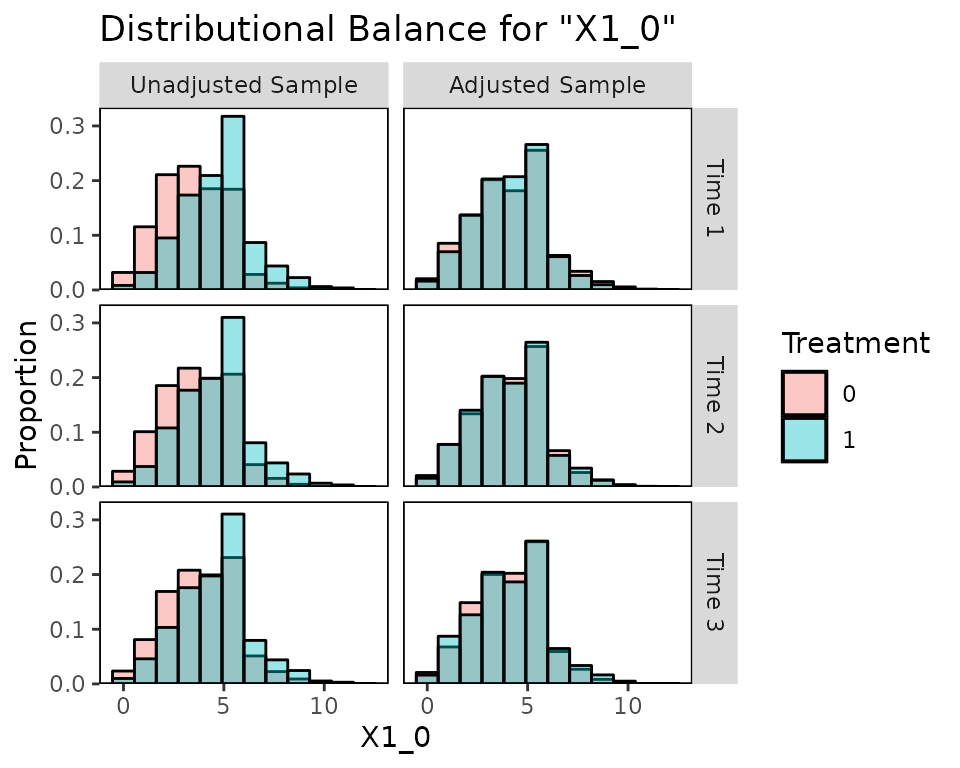

Balance for variables that only appear in certain time points will only be displayed at those time points:

bal.plot(Wmsm, var.name = "X2_1", which = "both")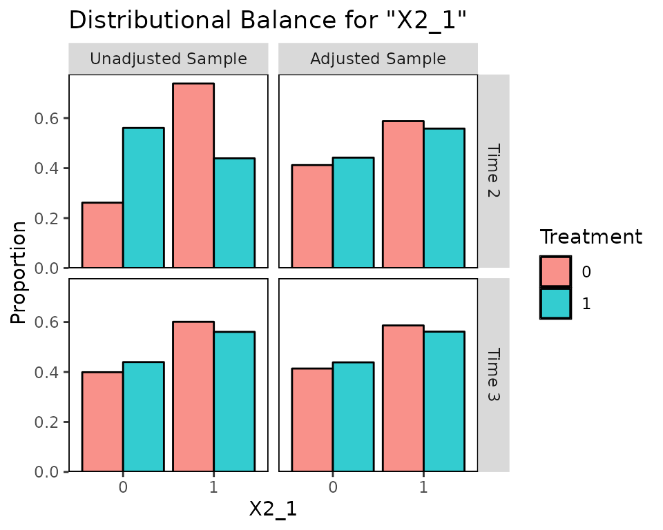

As with bal.tab(), which.time can be specified to limit output to chosen time points.

Finally, we’ll examine using love.plot() with longitudinal treatments to display balance for presentation.

`love.plot()`

love.plot() works with longitudinal treatments just as it does with point treatments, except that the user can choose whether to display separate plots for each time point or one plot with the summary across time points. As with bal.tab(), the user can set which.time to display only certain time points, including setting it to .all to display all time points (note that not all variables will be present in all time points). When set to .none (the default), the summary across time points is displayed. The agg.fun argument is set to "max" by default.

love.plot(Wmsm, binary = "std")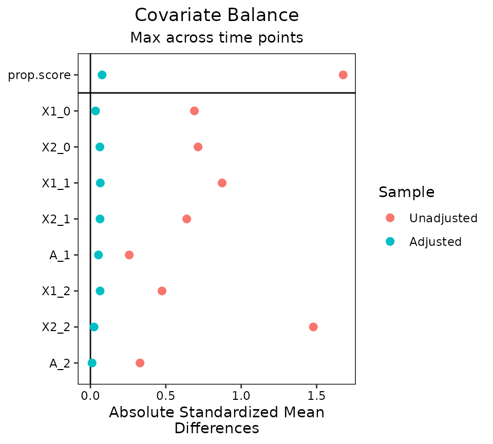

love.plot(Wmsm, binary = "std", which.time = .all)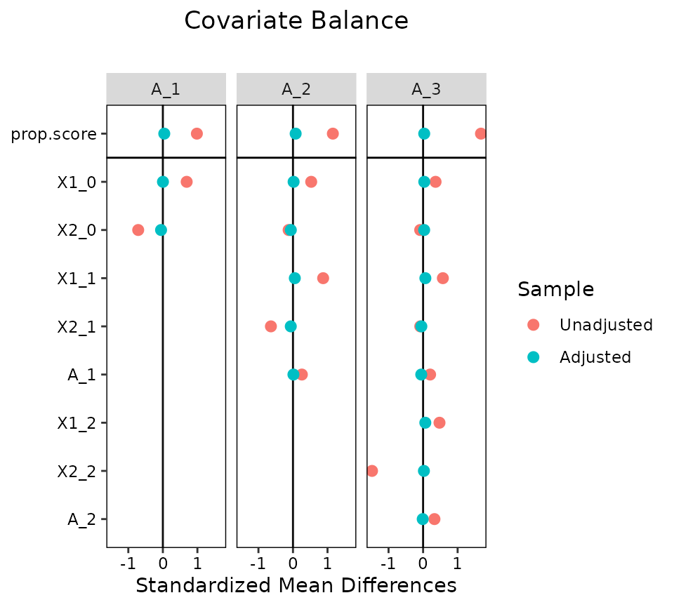

Censoring

Units often stop being observed partway through a study, which leaves later treatments and the outcome unrecorded for them. If dropout depends on treatment or covariate history, the units who remain are not representative of the sample that started, and weighting them to resemble it is the standard remedy (Robins et al. 1995; Hernán et al. 2000). The censoring model that produces those weights sits in the sequence alongside the treatment models, and its balance is assessed at the point where the censoring occurs.

A censoring indicator is marked with .cens() and follows the survival convention, in which 1 means the unit was censored and 0 means it is still under observation. It goes in the list of models at the position where it happens. Below we add an indicator of dropout after treatment period 2, so that A_3 is unobserved for the units it censors. Units with higher X1_2 and those treated at period 2 are more likely to drop out.

set.seed(100)
msmdata$C_2 <- rbinom(nrow(msmdata), 1,
                      prob = plogis(-4 + .35 * msmdata$X1_2 +
                                        .8 * msmdata$A_2))

#A_3 is not observed for the units censored after period 2
is.na(msmdata$A_3[msmdata$C_2 == 1]) <- TRUE

The list of formulas now has four entries for three treatment periods. The censoring model gets the same history as the treatment model that follows it.

bal.tab(list(A_1 ~ X1_0 + X2_0,
             A_2 ~ X1_1 + X2_1 +
               A_1 + X1_0 + X2_0,
             .cens(C_2) ~ X1_2 + X2_2 +
               A_2 + X1_1 + X2_1 +
               A_1 + X1_0 + X2_0,
             A_3 ~ X1_2 + X2_2 +
               A_2 + X1_1 + X2_1 +
               A_1 + X1_0 + X2_0),
        data = msmdata)

## Balance by Time Point
## 
## ─── 1. Treatment: A_1 
## 
## Balance Measures
##         Type Diff.Un
## X1_0 Contin.  0.6897
## X2_0  Binary -0.3253
## 
## Sample sizes
##     Control Treated
## All    3306    4194
## 
## ─── 2. Treatment: A_2 
## 
## Balance Measures
##         Type Diff.Un
## X1_1 Contin.  0.8736
## X2_1  Binary -0.2994
## A_1   Binary  0.1267
## X1_0 Contin.  0.5276
## X2_0  Binary -0.0599
## 
## Sample sizes
##     Control Treated
## All    3701    3799
## 
## ─── 3. Censoring: C_2 
## 
## Balance Measures
##         Type Diff.Un
## X1_2 Contin.  0.1991
## X2_2  Binary -0.0000
## A_2   Binary  0.0606
## X1_1 Contin.  0.1393
## X2_1  Binary -0.0207
## A_1   Binary  0.0206
## X1_0 Contin.  0.0752
## X2_0  Binary -0.0118
## 
## Sample sizes
##            Total
## Full        7500
## Uncensored  6158
## Censored    1342
## 
## ─── 4. Treatment: A_3 
## 
## Balance Measures
##         Type Diff.Un
## X1_2 Contin.  0.5003
## X2_2  Binary -0.5841
## A_2   Binary  0.1512
## X1_1 Contin.  0.5622
## X2_1  Binary -0.0437
## A_1   Binary  0.0936
## X1_0 Contin.  0.3534
## X2_0  Binary -0.0375
## 
## Sample sizes
##        0    1
## All 4126 2032

There is one table per entry, of whichever kind that entry’s model is. The first, second, and fourth are ordinary treatment balance tables; the third compares the units still under observation to the full sample at risk at that point, as described in the “Using cobalt with censoring” section of vignette("cobalt"). Its sample size table has a single column and reports how many units were at risk, how many remained, and how many were censored.

Two things about the third and fourth tables are worth pointing out. First, the fourth table is computed among the 6158 units still under observation, not all 7500: a unit censored at period 2 has no treatment at period 3 and nothing left to balance. Which units those are is worked out from the censoring indicators themselves, so it makes no difference whether the data leaves A_3 missing for them, as here, or records a value anyway. Second, no balance summary across time points is displayed, and neither is the collected table of sample sizes that normally accompanies it; each time point’s own table reports its sample sizes anyway. A censoring table and a treatment table describe different comparisons, so there is nothing meaningful to aggregate across them, just as there is nothing to aggregate across a mix of continuous and binary treatments. A list in which every entry is a censoring indicator is not a mixture and is summarized as usual.

weightitMSM() takes the same list and fits the censoring model along with the treatment models, returning a single set of weights that is their product.

Wmsm.cens <- weightitMSM(list(A_1 ~ X1_0 + X2_0,
                              A_2 ~ X1_1 + X2_1 +
                                A_1 + X1_0 + X2_0,
                              .cens(C_2) ~ X1_2 + X2_2 +
                                A_2 + X1_1 + X2_1 +
                                A_1 + X1_0 + X2_0,
                              A_3 ~ X1_2 + X2_2 +
                                A_2 + X1_1 + X2_1 +
                                A_1 + X1_0 + X2_0),
                         data = msmdata)

bal.tab(Wmsm.cens, un = TRUE, which.time = 3)

## Balance by Time Point
## 
## ─── 3. Censoring: C_2 ───────
## 
## Balance Measures
##         Type Diff.Un Diff.Adj
## X1_2 Contin.  0.1991   0.0623
## X2_2  Binary -0.0000  -0.0113
## A_2   Binary  0.0606   0.0112
## X1_1 Contin.  0.1393   0.0226
## X2_1  Binary -0.0207   0.0106
## A_1   Binary  0.0206   0.0657
## X1_0 Contin.  0.0752  -0.0095
## X2_0  Binary -0.0118  -0.0001
## 
## Effective sample sizes
##            Total
## Full        7500
## Uncensored  6158
## Adjusted    1495
## Censored    1342

Because the weights are the product across all four models, balance at any one time point is assessed with weights that include the others, censoring among them.

bal.plot() and love.plot() work here too. At a censoring time point, bal.plot() shows the weighted uncensored sample against the unweighted full sample rather than two treatment groups.

bal.plot(Wmsm.cens, var.name = "X1_2", which.time = 3,
         which = "both")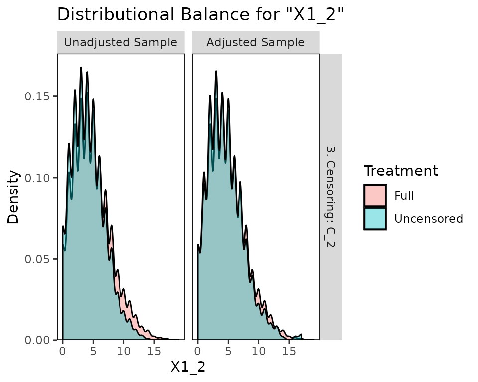

love.plot(Wmsm.cens, binary = "std", which.time = .all)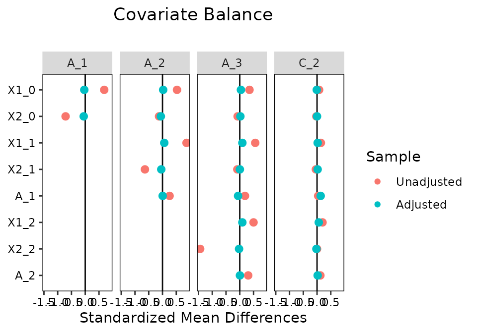

Other Packages

Here we used WeightIt to generate our MSM weights, but cobalt is compatible with other packages for longitudinal treatments as well. CBMSM objects from the CBPS package and iptw objects from the twang package can be used in place of the weightitMSM object in the above examples. In addition, users who have generated balancing weights outside any of these package can specify an argument to weights in bal.tab() with the formula or data frame methods to assess balance using those weights, or they can use the default method of bal.tab() to supply an object containing any of the objects required for balance assessment.

Note that CBPS estimates and assesses balance on MSM weights differently from twang and cobalt. Its focus is on ensuring balance across all treatment history permutations, whereas cobalt focuses on evaluating the similarity to sequential randomization. For this reason, it may appear that CBMSM objects have different balance qualities as measured by the two packages.

References

Cole, Stephen R., and Miguel A Hernán. 2008. “Constructing Inverse Probability Weights for Marginal Structural Models.” American Journal of Epidemiology 168 (6): 656–64. https://doi.org/10.1093/aje/kwn164.

Hernán, Miguel Ángel, Babette Brumback, and James M. Robins. 2000. “Marginal Structural Models to Estimate the Causal Effect of Zidovudine on the Survival of HIV-Positive Men.” Epidemiology 11 (5): 561–70. https://doi.org/10.1097/00001648-200009000-00012.

Jackson, John W. 2016. “Diagnostics for Confounding of Time-Varying and Other Joint Exposures:” Epidemiology 27 (6): 859–69. https://doi.org/10.1097/EDE.0000000000000547.

Robins, James M., Miguel Ángel Hernán, and Babette Brumback. 2000. “Marginal Structural Models and Causal Inference in Epidemiology.” Epidemiology 11 (5): 550–60. https://doi.org/10.1097/00001648-200009000-00011.

Robins, James M., Andrea Rotnitzky, and Lue Ping Zhao. 1995. “Analysis of Semiparametric Regression Models for Repeated Outcomes in the Presence of Missing Data.” Journal of the American Statistical Association 90 (429): 106–21. https://doi.org/10.1080/01621459.1995.10476493.

Thoemmes, Felix J., and Anthony D. Ong. 2016. “A Primer on Inverse Probability of Treatment Weighting and Marginal Structural Models.” Emerging Adulthood 4 (1): 40–59. https://doi.org/10.1177/2167696815621645.

VanderWeele, Tyler J., John W. Jackson, and Shanshan Li. 2016. “Causal Inference and Longitudinal Data: A Case Study of Religion and Mental Health.” Social Psychiatry and Psychiatric Epidemiology 51 (11): 1457–66. https://doi.org/10.1007/s00127-016-1281-9.

Noah Greifer