Using cobalt with Clustered, Multiply Imputed, and Other Segmented Data
Noah Greifer
2026-05-29
Source:vignettes/segmented-data.Rmd
segmented-data.RmdThis is a guide for the use of cobalt with more complicated data than is typical in studies using propensity scores and similar methods. In particular, this guide will explain cobalt’s features for handling multilevel or grouped data and data arising from multiple imputation. The features described here set cobalt apart from other packages that assess balance because they exist only in cobalt. It will be assumed that the basic functions of cobalt are understood; this guide will only address issues that are unique to these data scenarios.
cobalt and Segmented Data
First, let’s understand segmented data. Segmented data arises when the data involved in balance assessment needs to be split into segments to appropriately assess balance. These scenarios include clustered (e.g., multilevel) data, in which case balance should be assessed within each cluster; data arising from a sequential study, in which case balance should be assessed at each time point; multi-category treatments, in which case balance should be assessed for each pair of treatments; and multiply imputed data, in which case balance should be assessed within each imputation. cobalt can handle all these scenarios simultaneously, but how it does so may be a little complicated. This vignette explains how these scenarios are handled.
At the core is the idea that the most basic unit of balance
assessment is a balance statistic for a covariate. For binary treatments
or pairs of treatment levels, this can be the (standardized) mean
difference, Kolmogorov-Smirnoff (KS) statistic, etc. For continuous
treatments, this is the usually treatment-covariate correlation. These
statistics are generated by bal.tab() and can be plotted
using love.plot() when the data are not segmented. When the
data are segmented, these statistics need to be generated within each
segment. When the segmentation occurs in several ways in the same
dataset (e.g., with clustered and multiply imputed data, or with
longitudinal data with multi-category treatments), balance assessment
should reflect each layer of segmentation.
Although the idea of simply splitting data into segments is simple, there are a few options and limitations in cobalt that are important to consider. The basic idea is the same regardless of how the data are segmented: for each layer of segmentation, balance is assessed within segments of that layer, and the layers stack hierarchically. For example, for clustered and multiply imputed data, first the data are split by cluster; within each cluster, the data are split by imputation; balance statistics are computed within each imputation within each cluster. In some cases, a summary of balance across segments can be produced to simplify balance assessment. Matching and weighting are compatible with segmented data, but subclassification is its own special form of segmentation that is treated differently and will not be considered here.
Each of cobalt’s primary functions (bal.tab(),
bal.plot(), and love.plot()) has features to
handle segmented data sets. The following sections describe for each
data scenario the relevant features of each function. We’ll take a look
at a few common examples of segmented data: clustered data, multiply
imputed data, and multi-category and multiply imputed data. For
longitudinal treatments, see
vignette("longitudinal-treat").
Clustered Data
In clustered data, the data set must contain a variable denoting the
group each individual belongs to. This may be a group considered a
nuisance that must be accounted for to eliminate confounding (e.g.,
hospitals in a multi-site medical treatment study), or a group of
concern for effect moderation (e.g., race or gender). In the examples
below, we will imagine that we are interested in the ATT of
treat on re78 stratified by race.
Thus, we will condition on the propensity score within each cluster.
First, let’s estimate propensity scores and perform matching within each race group. We can do this by performing separate analyses within each cluster, but we can also use exact matching in MatchIt to ensure matches occur within clusters. It is important to note that this analysis does not necessarily represent a sound statistical analysis and is being used for illustrative purposes only.
library("cobalt")
data("lalonde", package = "cobalt")

library("MatchIt")
m.out <- matchit(treat ~ race * (age + educ + married + nodegree + re74 + re75),
                 data = lalonde,
                 method = "nearest",
                 exact = "race",
                 replace = TRUE,
                 ratio = 2)
bal.tab()
The output produced by bal.tab() with clustered data
contains balance tables for each cluster and a summary of balance across
clusters. To use bal.tab() with groups, there are four
arguments that should be considered. These are cluster,
which.cluster, cluster.summary, and
cluster.fun.
clusteris a vector of group membership for each unit or the name of a variable in a provided data set containing group membership.which.clusterdetermines for which clusters balance tables are to be displayed, if any. (Default: display all clusters)cluster.summarydetermines whether the cluster summary is to be displayed or not. (Default: hide the cluster summary)cluster.fundetermines which function(s) are used to combine balance statistics across clusters for the cluster summary. (Default: whenabs = FALSE, minimum, mean, and maximum; whenabs = TRUE, mean and maximum)
The arguments are in addition to the other arguments that are used
with bal.tab() to display balance.
cluster.summary and cluster.fun can also be
set as global options by using set.cobalt.options(). Let’s
examine balance on our data within each race group.
bal.tab(m.out, cluster = "race")## Balance by cluster
##
## - - - Cluster: black - - -
## Balance Measures
## Type Diff.Adj
## distance Distance 0.0150
## age Contin. -0.1001
## educ Contin. 0.0794
## married Binary 0.0288
## nodegree Binary -0.0032
## re74 Contin. -0.1501
## re75 Contin. -0.1406
##
## Sample sizes
## 0 1
## All 87. 156
## Matched (ESS) 41.53 156
## Matched (Unweighted) 76. 156
## Unmatched 11. 0
##
## - - - Cluster: hispan - - -
## Balance Measures
## Type Diff.Adj
## distance Distance 0.0947
## age Contin. 0.1914
## educ Contin. -0.4159
## married Binary 0.1364
## nodegree Binary 0.2273
## re74 Contin. 0.1161
## re75 Contin. 0.0683
##
## Sample sizes
## 0 1
## All 61. 11
## Matched (ESS) 15.12 11
## Matched (Unweighted) 18. 11
## Unmatched 43. 0
##
## - - - Cluster: white - - -
## Balance Measures
## Type Diff.Adj
## distance Distance 0.0216
## age Contin. -0.4201
## educ Contin. -0.1403
## married Binary -0.0556
## nodegree Binary 0.1111
## re74 Contin. -0.0417
## re75 Contin. 0.0298
##
## Sample sizes
## 0 1
## All 281. 18
## Matched (ESS) 25.92 18
## Matched (Unweighted) 31. 18
## Unmatched 250. 0
## - - - - - - - - - - - - - -Here we see balance tables for each cluster. These are the same
output we would see if we use bal.tab() for each cluster
separately (e.g., using the subset argument). All the
commands that work for bal.tab() also work here with the
same results. Next, we can request a balance summary across clusters and
hide the individual clusters by setting
which.cluster = .none:
bal.tab(m.out, cluster = "race", which.cluster = .none)## Balance summary across all clusters
## Type Min.Diff.Adj Mean.Diff.Adj Max.Diff.Adj
## distance Distance 0.0150 0.0438 0.0947
## age Contin. -0.4201 -0.1096 0.1914
## educ Contin. -0.4159 -0.1590 0.0794
## married Binary -0.0556 0.0366 0.1364
## nodegree Binary -0.0032 0.1117 0.2273
## re74 Contin. -0.1501 -0.0252 0.1161
## re75 Contin. -0.1406 -0.0142 0.0683
##
## Total sample sizes across clusters
## 0 1
## All 429. 185
## Matched (ESS) 82.57 185
## Matched (Unweighted) 125. 185
## Unmatched 304. 0This table presents the minimum, mean, and maximum balance statistics
for each variable across clusters. Setting un = TRUE will
also display the same values for the adjusted data set. Setting
abs = TRUE requests summaries of absolute balance
statistics which displays the extremeness of balance statistics for each
variable; thus, if, for example, in some groups there are large negative
mean differences and in other groups there are large positive mean
differences, this table will display large mean differences, even though
the average mean difference is close to 0. While it’s important to know
the average balance statistic overall, assessing the absolute balance
statistics provides more information about balance within each cluster
rather than in aggregate.
To examine balance for just a few clusters at a time, users can enter
values for which.cluster. This can be a vector of clusters
indices (i.e., 1, 2, 3, etc.) or names (e.g., “black”, “hispan”,
“white”). Users also specify which.cluster = .none as above
to omit cluster balance for all clusters and just see the summary across
clusters. Users can force display of the summary across clusters by
specifying TRUE or FALSE for
cluster.summary. When which.cluster = .none,
cluster.summary will automatically be set to
TRUE (or else there wouldn’t be any output!). When
examining balance within a few groups, it can be more helpful to examine
balance within each group and ignore the summary. Below are examples of
the use of which.cluster and cluster.summary
to change bal.tab() output.
#Just for black
bal.tab(m.out, cluster = "race", which.cluster = "black")
## Balance by cluster
##
## - - - Cluster: black - - -
## Balance Measures
## Type Diff.Adj
## distance Distance 0.0150
## age Contin. -0.1001
## educ Contin. 0.0794
## married Binary 0.0288
## nodegree Binary -0.0032
## re74 Contin. -0.1501
## re75 Contin. -0.1406
##
## Sample sizes
## 0 1
## All 87. 156
## Matched (ESS) 41.53 156
## Matched (Unweighted) 76. 156
## Unmatched 11. 0
## - - - - - - - - - - - - - -
#Just the balance summary across clusters with only the mean
bal.tab(m.out, cluster = "race", which.cluster = .none,
        cluster.fun = "mean")
## Balance summary across all clusters
## Type Mean.Diff.Adj
## distance Distance 0.0438
## age Contin. -0.1096
## educ Contin. -0.1590
## married Binary 0.0366
## nodegree Binary 0.1117
## re74 Contin. -0.0252
## re75 Contin. -0.0142
##
## Total sample sizes across clusters
## 0 1
## All 429. 185
## Matched (ESS) 82.57 185
## Matched (Unweighted) 125. 185
## Unmatched 304. 0These can also be set as global options by using, for example,
set.cobalt.options(cluster.fun = "mean"), which allows
users not to type a non-default option every time they call
bal.tab().
bal.plot()
bal.plot() functions as it does with non-clustered data,
except that multiple plots can be produced at the same time displaying
balance for each cluster. The arguments to bal.plot() are
the same as those for bal.tab(), except that
cluster.summary is absent. Below is an example of the use
of bal.plot() with clustered data:
bal.plot(m.out, var.name = "age", cluster = "race", which = "both")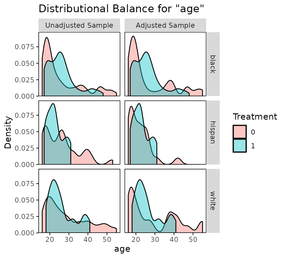
Balance plots for each cluster are displayed next to each other. You
can specify which.cluster as with bal.tab() to
restrict plotting to a subset of clusters.
love.plot()
love.plot() shines with clustered data because there are
several options that are unique to cobalt and help with the
visual display of balance. One way to display cluster balance with
love.plot() is to produce different plots for each cluster,
as bal.plot() does. This method should not be used with
many clusters, or the plots will be unreadable. In our present example,
this is not an issue. To do so, the which.cluster argument
in bal.tab() or love.plot() must be set to the
names or indices of the clusters for which balance is to be plotted. If
which.cluster is set to .all (the default),
all clusters will be plotted. Below is an example:
love.plot(m.out, cluster = "race")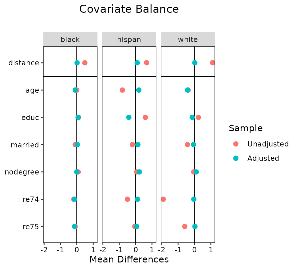
These plots function like those from using love.plot()
with non-clustered data, except that they cannot be sorted based on the
values of the balance statistics (they can still be sorted
alphabetically, though). This is to ensure that the covariates line up
across the plots. The same axis limits will apply to all plots.
Second, balance can be displayed summarizing across clusters by
plotting an aggregate function (i.e., the mean or maximum) of the
balance statistic for each covariate across clusters. To do this,
which.cluster in the love.plot command must be
set to .none. To change which aggregate function is
displayed, use the argument to agg.fun, which may be “mean”
or “max”. Below is an example:
love.plot(m.out, cluster = "race",
          which.cluster = .none,
          agg.fun = "mean")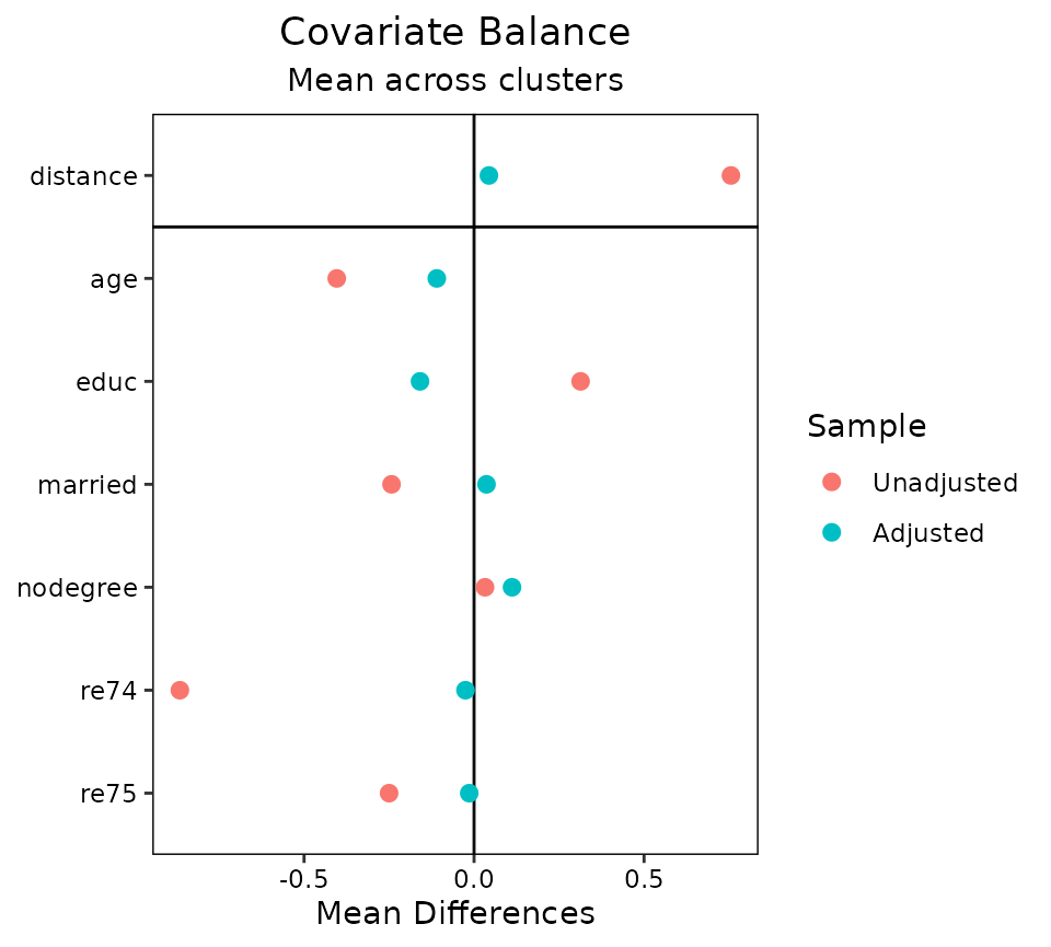
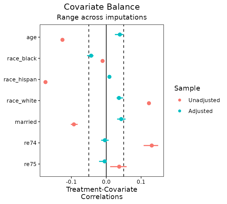
A third option is to set agg.fun = "range" (the
default), which produces a similar plot as above except that the minimum
and maximum values of the balance statistics for each covariate are
displayed as well. See below for an example:
love.plot(m.out, cluster = "race", which.cluster = .none, agg.fun = "range")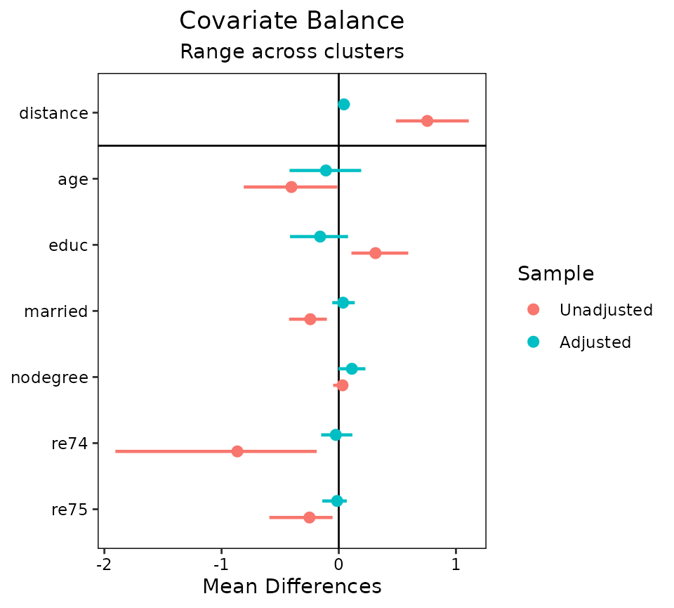
Each point represents the mean balance statistic, and the bars
represent intervals bounded by the minimum and maximum of each balance
statistic. This display can be especially helpful with many clusters
given that the mean alone may not tell the whole story. In some cases,
it might be useful to set limits on the x-axis by using the
limits argument in love.plot(); doing so may
cut off some of the ranges, but whatever is left will be displayed. All
love.plot() arguments work with these methods as they do in
the case of non-clustered data. When var.order is specified
as "unadjusted" or "adjusted", the ordering
will occur on the mean balance statistic when using
agg.fun = "range". Only one argument to stats
is allowed when segmented data produces more than one plot (i.e., as it
would with which.cluster = .all).
Multiply Imputed Data
Multiply imputed data works in a very similar way to clustered data, except the “grouping” variable refers to imputations rather than clusters. Thus, each row belongs to one imputation (i.e., the data set should be in “long” format). The data set used should only include the imputed data sets and not the original data set with missing values. The imputed data sets can be of different sizes (i.e., because matching reduced the size of each differently), but it is preferred that they are the same size and weights are used to indicate which units belong to the sample and which do not.
In the example below, we will use a version of the Lalonde data set
with some values missing. We will use the mice package to
implement multiple imputation with chained equations. We will perform
the “within” approach using the MatchThem to perform propensity
score weighting within each imputation with educ as the
continuous treatment (substantively this analysis makes no sense and is
just for illustration).
data("lalonde_mis", package = "cobalt")
set.seed(100)

#Generate imputed data sets
m <- 10 #number of imputed data sets
imp.out <- mice::mice(lalonde_mis, m = m, print = FALSE)


#Performing generalized propensity score weighting in each imputation
wt.out <- MatchThem::weightthem(educ ~ age + race + married +
                                    re74 + re75, datasets = imp.out,
                                approach = "within", method = "glm")
bal.tab()
There are a few ways to use bal.tab() with our imputed
data sets. When using the mimids or wimids
methods for MatchThem objects, only the output object needs to
be supplied. When using other methods, an argument to imp
can be supplied; this should contain the imputation identifiers for each
unit or the name of a variable in a supplied dataset (e.g., through the
data argument) that contains the imputation identifiers.
Alternatively, the mids object resulting from the call to
mice can be supplied to the data argument, which
automatically populates imp. There are four arguments that
are only relevant to imputed data:
impis a vector of imputation numbers for each unit or the name of a variable in an available data set containing the imputation numbers. Ifdatais amidsobject or if themimidsorwimidsmethods are used, this doesn’t need to be specified.which.impdetermines for which imputation balance assessment is to be displayed. Often it can be useful to examine balance in just a few imputations for a detailed examination of what is going on. Can be.allto display all imputations (not recommended),.noneto display none, or a vector providing the imputation numbers for the desired imputations. (Default: no imputations are displayed.)imp.summarydetermines whether to display a summary of balance across imputations. (Default: the summary of balance across imputations is displayed.)imp.fundetermines which function(s) are used to combine balance statistics across imputations for the summary of balance across imputations. (Default: whenabs = FALSE, minimum, mean, and maximum; whenabs = TRUE, mean and maximum)
imp.summary and imp.fun can also be set as
global options by using set.cobalt.options() like the
corresponding cluster options.
In many cases, not all variables are imputed, and often the treatment
variable is not imputed. If each imputation has the same number of
units, you can specify other arguments (e.g., treatment, distance) by
specifying an object of the length of one imputation, and this vector
will be applied to all imputations. This will come in handy when
supplying additional covariates that weren’t involved in the imputation
or propensity score estimation through addl. To do this,
the imputed data set must be sorted by imputation and unit ID.
Because we’re using a wimids object, we can just call
bal.tab() with it as the first argument.
#Checking balance on the output object
bal.tab(wt.out)
## Balance summary across all imputations
## Type Min.Corr.Adj Mean.Corr.Adj Max.Corr.Adj
## age Contin. 0.0248 0.0390 0.0488
## race_black Binary -0.0550 -0.0433 -0.0366
## race_hispan Binary 0.0066 0.0091 0.0118
## race_white Binary 0.0297 0.0365 0.0481
## married Binary 0.0312 0.0429 0.0553
## re74 Contin. -0.0147 -0.0039 0.0071
## re75 Contin. -0.0206 -0.0046 0.0016
##
## Average effective sample sizes across imputations
## Total
## Unadjusted 614.
## Adjusted 541.56First, we see a balance summary across all the imputations. This
table presents the minimum, mean, and maximum balance statistics for
each variable across imputations. Setting un = TRUE will
also display the same values for the adjusted data set. Setting
abs = TRUE will make bal.tab() report
summaries of the absolute values of the balance statistics. This table
functions in the same way as the table for balance across clusters.
Below is the average sample size across imputations; in some matching
and weighting schemes, the sample size (or effective sample size) may
differ across imputations.
When requesting the balance summary across imputations, the
thresholds argument needs special care. Because multiple
balance summaries are produced for each covariate by default, simply
supplying thresholds is not enough to identify which
summary of the balance statistics across imputations is the one for
which the threshold is to be applied. The solution to this is to use
imp.fun to specify which summary is desired; the threshold
will be applied to that summary. For example, to request a threshold on
the maximum absolute treatment-covariate correlation across imputations,
you could run
## Balance summary across all imputations
##                Type Max.Corr.Adj         R.Threshold
## age         Contin.       0.0488     Balanced, <0.05
## race_black   Binary       0.0550 Not Balanced, >0.05
## race_hispan  Binary       0.0118     Balanced, <0.05
## race_white   Binary       0.0481     Balanced, <0.05
## married      Binary       0.0553 Not Balanced, >0.05
## re74        Contin.       0.0147     Balanced, <0.05
## re75        Contin.       0.0206     Balanced, <0.05
##
## Balance tally for treatment correlations
##                     count
## Balanced, <0.05         5
## Not Balanced, >0.05     2
##
## Variable with the greatest treatment correlation
##  Variable Max.Corr.Adj         R.Threshold
##   married       0.0553 Not Balanced, >0.05
##
## Average effective sample sizes across imputations
##             Total
## Unadjusted 614.
## Adjusted   541.56
To view balance on individual imputations, you can specify an
imputation number to which.imp. (The summary across
imputations is automatically hidden but can be forced to be displayed
using imp.summary.)
bal.tab(wt.out, which.imp = 1)## Balance by imputation
##
## - - - Imputation 1 - - -
## Balance Measures
## Type Corr.Adj
## age Contin. 0.0488
## race_black Binary -0.0550
## race_hispan Binary 0.0089
## race_white Binary 0.0481
## married Binary 0.0463
## re74 Contin. 0.0023
## re75 Contin. -0.0011
##
## Effective sample sizes
## Total
## Unadjusted 614.
## Adjusted 530.63
## - - - - - - - - - - - - - -As with clustered data, all bal.tab() options work as
with non-imputed data. Indeed, the functions for clustered and imputed
data are nearly identical except that for imputed data,
bal.tab() computes the average sample size across
imputations, whereas for other forms of segmented data,
bal.tab() computes the total sample size across groups.
bal.plot()
bal.plot() works with imputed data as it does with
non-imputed data, except that multiple plots can be produced displaying
balance for multiple imputations at a time. The arguments to
bal.plot() are the same as those for
bal.tab(), except that imp.summary is absent.
Below is an example of the use of bal.plot() with imputed
and weighted data from MatchThem, examining balance in the
first imputation:
bal.plot(wt.out, which.imp = 1, var.name = "age", which = "both")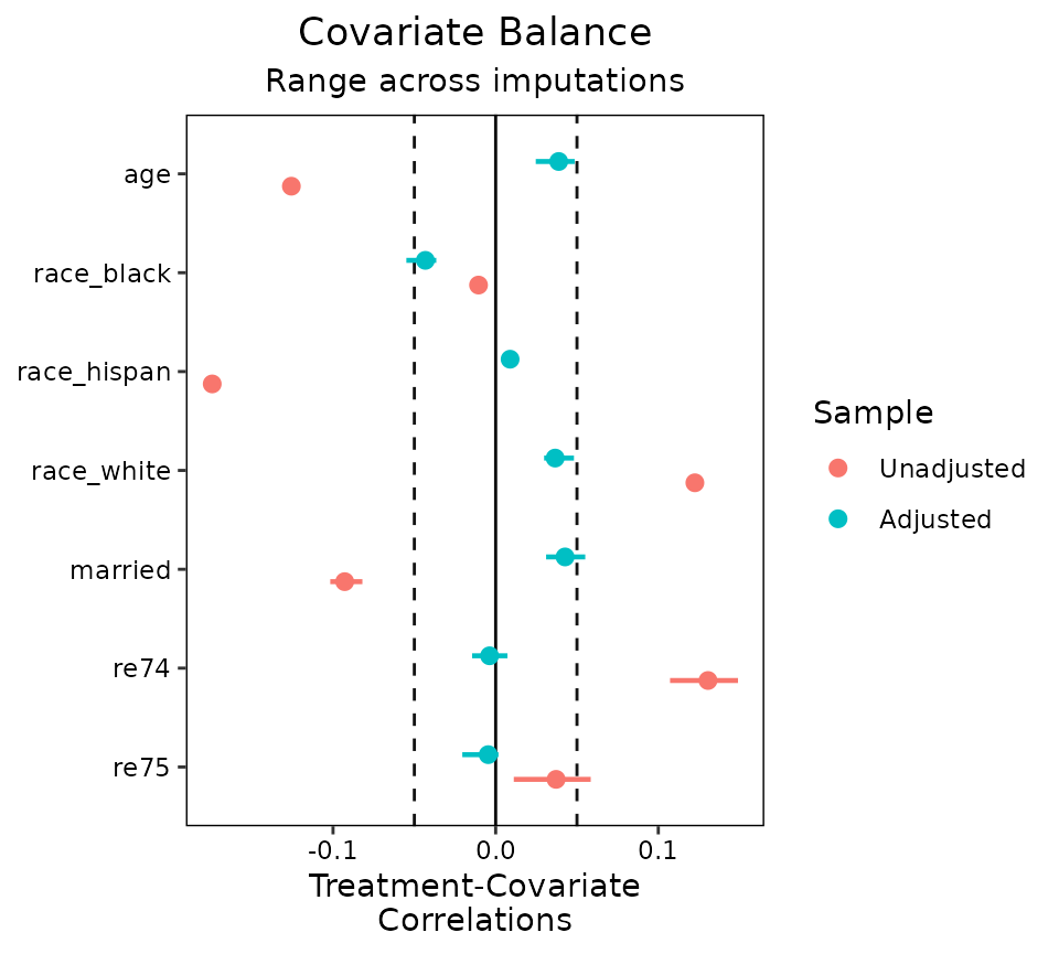
When many imputations are generated, it is recommended not to plot
all at the same time by specifying an argument to
which.imp, as done above. When which.imp is
set to .none, data are combined across imputation to
produce a single plot, which can act as a summary heuristic but which
may obscure imbalances occurring in only a few imputations and not
others.
love.plot()
love.plot() functions with imputed data as it does with
clustered data. It is not recommended to display balance for multiple
imputations at a time, and rather to display balance summarized across
imputations:
Often these ranges will be small if the imputed data sets are very
similar to each other, but the more imputations are generated, the wider
the ranges tend to be. Unlike with bal.tab(),
thresholds can be used with love.plot()
without specifying an argument to agg.fun.
Multi-Category Treatments with Multiply Imputed Data
So far we’ve seen how cobalt functions work with one layer of data segmentation, but now let’s see what it’s like to work with two or more layers of segmentation. As an example, we’ll first look at multiply imputed data with a multi-category treatment. With multi-category treatments, balance is typically assessed by examining balance statistics computed for pairs of treatments. With multi-category and multiply imputed data, the data is segmented both by imputation and by treatment pair.
We’ll use the three-category race variable as our
multi-category treatment and use the same imputed data as above. Again,
the MatchThem package can be used to estimate weights in
multiply imputed data. We’ll use propensity score weighting to estimate
the ATE of race. As before, this analysis makes no sense
substantively and is just for illustration.
#Estimate weights within each imputation using propensity scores
wt3.out <- MatchThem::weightthem(race ~ age + educ + married +
                                     nodegree + re74 + re75,
                                 datasets = imp.out, approach = "within",
                                 method = "glm", estimand = "ATE")
bal.tab()
Using bal.tab() on the resulting object does the
following: for each pair of treatments, balance is assessed for each
imputation and aggregated across imputations. That is, for each pair of
treatments, everything described in the previous section will occur.
bal.tab(wt3.out)## Balance by treatment pair
##
## - - - black (0) vs. hispan (1) - - -
## Balance summary across all imputations
## Type Min.Diff.Adj Mean.Diff.Adj Max.Diff.Adj
## age Contin. -0.0113 0.0133 0.0261
## educ Contin. -0.1193 -0.1034 -0.0738
## married Binary -0.0420 -0.0321 -0.0250
## nodegree Binary 0.0385 0.0501 0.0563
## re74 Contin. -0.1112 -0.0779 -0.0254
## re75 Contin. -0.1134 -0.0881 -0.0574
##
## Average effective sample sizes across imputations
## black hispan
## Unadjusted 243. 72.
## Adjusted 157.22 55.7
##
## - - - black (0) vs. white (1) - - -
## Balance summary across all imputations
## Type Min.Diff.Adj Mean.Diff.Adj Max.Diff.Adj
## age Contin. 0.0209 0.0353 0.0494
## educ Contin. -0.0714 -0.0574 -0.0291
## married Binary -0.0001 0.0054 0.0105
## nodegree Binary 0.0118 0.0192 0.0231
## re74 Contin. -0.1350 -0.1062 -0.0882
## re75 Contin. -0.1213 -0.1044 -0.0895
##
## Average effective sample sizes across imputations
## black white
## Unadjusted 243. 299.
## Adjusted 157.22 260.72
##
## - - - hispan (0) vs. white (1) - - -
## Balance summary across all imputations
## Type Min.Diff.Adj Mean.Diff.Adj Max.Diff.Adj
## age Contin. 0.0122 0.0220 0.0399
## educ Contin. 0.0375 0.0460 0.0524
## married Binary 0.0315 0.0375 0.0448
## nodegree Binary -0.0337 -0.0310 -0.0224
## re74 Contin. -0.0628 -0.0282 0.0030
## re75 Contin. -0.0401 -0.0163 0.0107
##
## Average effective sample sizes across imputations
## hispan white
## Unadjusted 72. 299.
## Adjusted 55.7 260.72
## - - - - - - - - - - - - - - - - - - - - - - - -Other options can be supplied to choose how balance is computed with
multi-category treatments; these are described at
?bal.tab.multi and in the main vignette. Importantly,
though, a balance summary across treatment pairs is not available.
bal.plot()
bal.plot() works with multi-category treatments the same
way it does with binary treatments. All treatment levels are displayed
on the same plot. As before, with multiply imputed data, balance can be
examined on one or more imputations at a time.
bal.plot(wt3.out, var.name = "married", which.imp = 1,
         which = "both")
love.plot()
With multiple layers of segmentation, love.plot() has a
few options. Before, we saw that we could facet the plot by the segments
or aggregate across segments; with multiple layers, we can do both.
love.plot() can aggregate across as many layers as there
are and can facet with segments of one layer. With more than two layers
of segmentation, at least one of the which. arguments must
be .none (to aggregate) or of length 1 (to facet at one
segment of the layer). Here we’ll demonstrate aggregating across
imputations while faceting on treatment pairs.
love.plot(wt3.out, threshold = .1, agg.fun = "mean")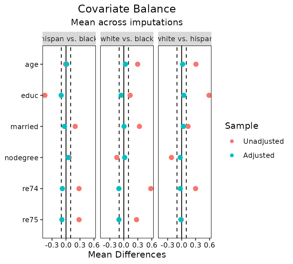
The arguments to which.treat, which.imp,
abs, and agg.fun can be used to control how
the plots are faceted and aggregated as they can with single-layer
data.
Concluding Remarks
We have demonstrated the use of cobalt with clustered data,
multiply imputed data, and multiply imputed data with a multi-category
treatment. Though there are few published recommendations for the
display of balance in some of these cases, we believe these tools may
encourage development in this area. In general, we believe in displaying
the most relevant information as compactly as possible, and thus
recommend using love.plot() with some degree of aggregation
for inclusion in published work.