
This function extracts variable names from a bal.tab object for use in specifying alternate variable names in bal.tab(), print(), format(), as.data.frame(), and love.plot(). Optionally, a file can be written for easy editing of names.
Arguments
- b
a
bal.tabobject; the output of a call tobal.tab().- type
the type of output desired. Can either be
"df"for a data frame or"vec"for a named vector. See "Value". The default is"vec"unlessfileis notNULL.- file
optional; a file name to save the output if
type = "df". Seeutils::write.csv(), whichvar.name()calls. Must end in.csv.- minimal
whether the output should contain all variable names (i.e., all rows that appear the output of
bal.tab()) or just the unique base variables. See "Details".
Value
If type = "vec", a character vector with the variable names as the names and the names they are displayed under as the entries.
If type = "df", a data frame with two columns called "old" and "new", the first with the variable names and the second with the names they are displayed under.
When no var.names has been applied to the object, every variable is displayed as it is stored and the two agree. When one has, the names it produced are given, so that they can be edited rather than written out again; see Details.
If file is not NULL, the output will be returned invisibly.
Details
The purpose of the function is to make supplying new variable names to the var.names argument easier. Rather than manually creating a vector or data frame with all the variable names that one desires to change, one can use var.names() to extract variable names from a bal.tab object and edit the output. Importantly, the output can be saved to a CSV file, which can be easily edited and read back into R, as demonstrated in the Example. See display-options for what var.names does and for the structures it accepts.
When minimal = TRUE, only a minimal set of variables will be output. For example, if the variables analyzed in bal.tab() are age, race, and married, and int = TRUE in bal.tab(), many variables will appear in the output, including expansions of the factor variables, the polynomial terms, and the interactions. Rather than renaming all of these variables individually, one can rename just the three base variables, and all variables that arise from them will be accordingly renamed. Setting minimal = TRUE requests only these base variables.
If a var.names was given in the call to bal.tab(), the names it produced are what is returned, so that a set of names arrived at once can be edited rather than written out again. Passing the result back to any of the functions that take var.names reproduces the names it came from, because the old names it is keyed by are the ones the variables are stored under, which var.names never changes.
Which names an edit then reaches follows from minimal, as it does for any var.names: an edit to a base variable in the minimal output reaches every name that variable appears in, while an edit to an entry of the full output changes only the name it is an entry for.
Note
Not all programs can properly read the Unicode characters for the polynomial terms when requested. These may appear strange in, e.g., Excel, but R will process the characters correctly.
See also
display-options for var.names, the argument this function supplies
Examples
data(lalonde, package = "cobalt")
b1 <- bal.tab(treat ~ age + race + married, data = lalonde,
int = TRUE)
#> Note: `s.d.denom` not specified; assuming "pooled".
v1 <- var.names(b1, type = "vec", minimal = TRUE)
v1["age"] <- "Age (Years)"
v1["race"] <- "Race/Eth"
v1["married"] <- "Married"
love.plot(b1, var.names = v1, factor_sep = ": ")
#> Warning: Standardized mean differences and raw mean differences are present in the same
#> plot. Use the `stars` argument to distinguish between them and appropriately
#> label the x-axis. See ?love.plot (`?cobalt::love.plot()`) for details.
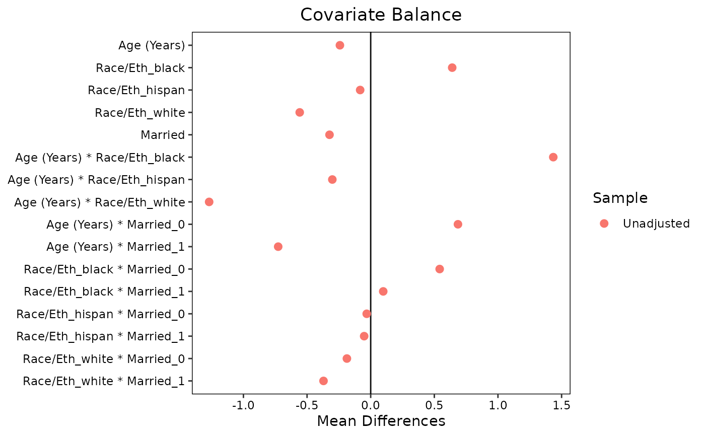 #The same names in the table, set once in `bal.tab()`
b1 <- bal.tab(treat ~ age + race + married, data = lalonde,
int = TRUE, var.names = v1)
#> Note: `s.d.denom` not specified; assuming "pooled".
b1
#> Balance Measures
#> Type Diff.Un
#> Age (Years) Contin. -0.2419
#> Race/Eth_black Binary 0.6404
#> Race/Eth_hispan Binary -0.0827
#> Race/Eth_white Binary -0.5577
#> Married Binary -0.3236
#> Age (Years) * Race/Eth_black Contin. 1.4347
#> Age (Years) * Race/Eth_hispan Contin. -0.3015
#> Age (Years) * Race/Eth_white Contin. -1.2694
#> Age (Years) * Married_0 Contin. 0.6856
#> Age (Years) * Married_1 Contin. -0.7269
#> Race/Eth_black * Married_0 Binary 0.5420
#> Race/Eth_black * Married_1 Binary 0.0985
#> Race/Eth_hispan * Married_0 Binary -0.0313
#> Race/Eth_hispan * Married_1 Binary -0.0514
#> Race/Eth_white * Married_0 Binary -0.1870
#> Race/Eth_white * Married_1 Binary -0.3707
#>
#> Sample sizes
#> Control Treated
#> All 429 185
#They come back out to be edited rather than rewritten
v1 <- var.names(b1, type = "vec", minimal = TRUE)
v1
#> age race married
#> "Age (Years)" "Race/Eth" "Married"
v1["married"] <- "Married at baseline"
print(b1, var.names = v1)
#> Balance Measures
#> Type Diff.Un
#> Age (Years) Contin. -0.2419
#> Race/Eth_black Binary 0.6404
#> Race/Eth_hispan Binary -0.0827
#> Race/Eth_white Binary -0.5577
#> Married at baseline Binary -0.3236
#> Age (Years) * Race/Eth_black Contin. 1.4347
#> Age (Years) * Race/Eth_hispan Contin. -0.3015
#> Age (Years) * Race/Eth_white Contin. -1.2694
#> Age (Years) * Married at baseline_0 Contin. 0.6856
#> Age (Years) * Married at baseline_1 Contin. -0.7269
#> Race/Eth_black * Married at baseline_0 Binary 0.5420
#> Race/Eth_black * Married at baseline_1 Binary 0.0985
#> Race/Eth_hispan * Married at baseline_0 Binary -0.0313
#> Race/Eth_hispan * Married at baseline_1 Binary -0.0514
#> Race/Eth_white * Married at baseline_0 Binary -0.1870
#> Race/Eth_white * Married at baseline_1 Binary -0.3707
#>
#> Sample sizes
#> Control Treated
#> All 429 185
if (FALSE) { # \dontrun{
b2 <- bal.tab(treat ~ age + race + married + educ + nodegree +
re74 + re75 + I(re74==0) + I(re75==0),
data = lalonde)
var.names(b2, file = "varnames.csv")
##Manually edit the CSV (e.g., in Excel), then save it.
v2 <- read.csv("varnames.csv")
love.plot(b2, var.names = v2)
} # }
#The same names in the table, set once in `bal.tab()`
b1 <- bal.tab(treat ~ age + race + married, data = lalonde,
int = TRUE, var.names = v1)
#> Note: `s.d.denom` not specified; assuming "pooled".
b1
#> Balance Measures
#> Type Diff.Un
#> Age (Years) Contin. -0.2419
#> Race/Eth_black Binary 0.6404
#> Race/Eth_hispan Binary -0.0827
#> Race/Eth_white Binary -0.5577
#> Married Binary -0.3236
#> Age (Years) * Race/Eth_black Contin. 1.4347
#> Age (Years) * Race/Eth_hispan Contin. -0.3015
#> Age (Years) * Race/Eth_white Contin. -1.2694
#> Age (Years) * Married_0 Contin. 0.6856
#> Age (Years) * Married_1 Contin. -0.7269
#> Race/Eth_black * Married_0 Binary 0.5420
#> Race/Eth_black * Married_1 Binary 0.0985
#> Race/Eth_hispan * Married_0 Binary -0.0313
#> Race/Eth_hispan * Married_1 Binary -0.0514
#> Race/Eth_white * Married_0 Binary -0.1870
#> Race/Eth_white * Married_1 Binary -0.3707
#>
#> Sample sizes
#> Control Treated
#> All 429 185
#They come back out to be edited rather than rewritten
v1 <- var.names(b1, type = "vec", minimal = TRUE)
v1
#> age race married
#> "Age (Years)" "Race/Eth" "Married"
v1["married"] <- "Married at baseline"
print(b1, var.names = v1)
#> Balance Measures
#> Type Diff.Un
#> Age (Years) Contin. -0.2419
#> Race/Eth_black Binary 0.6404
#> Race/Eth_hispan Binary -0.0827
#> Race/Eth_white Binary -0.5577
#> Married at baseline Binary -0.3236
#> Age (Years) * Race/Eth_black Contin. 1.4347
#> Age (Years) * Race/Eth_hispan Contin. -0.3015
#> Age (Years) * Race/Eth_white Contin. -1.2694
#> Age (Years) * Married at baseline_0 Contin. 0.6856
#> Age (Years) * Married at baseline_1 Contin. -0.7269
#> Race/Eth_black * Married at baseline_0 Binary 0.5420
#> Race/Eth_black * Married at baseline_1 Binary 0.0985
#> Race/Eth_hispan * Married at baseline_0 Binary -0.0313
#> Race/Eth_hispan * Married at baseline_1 Binary -0.0514
#> Race/Eth_white * Married at baseline_0 Binary -0.1870
#> Race/Eth_white * Married at baseline_1 Binary -0.3707
#>
#> Sample sizes
#> Control Treated
#> All 429 185
if (FALSE) { # \dontrun{
b2 <- bal.tab(treat ~ age + race + married + educ + nodegree +
re74 + re75 + I(re74==0) + I(re75==0),
data = lalonde)
var.names(b2, file = "varnames.csv")
##Manually edit the CSV (e.g., in Excel), then save it.
v2 <- read.csv("varnames.csv")
love.plot(b2, var.names = v2)
} # }