Response families in bartisan

Noah Greifer

2026-09-15

library(bartisan)

set.seed(2026)

# Small chains throughout, so that this vignette builds quickly. The defaults
# are 50 trees and 800 draws after 200 warmup iterations.
ctrl <- bartisan_control(num_trees = 10, num_burn = 150, num_draws = 150)

Introduction

This vignette is about choosing a family for bartisan(). It covers what each one assumes, when to prefer it over the alternatives, and the handful of places where the choice has a consequence that is easy to miss. ?bartisan_control covers how the sampler goes about fitting them.

family works the way it does in glm(): the stats::family objects work unchanged, bartisan adds the families that have no glm() counterpart in the same style, and custom_family() takes a log density written as an R function when nothing on the list fits. Unlike ordinary BART, nothing here requires the response to be conditionally conjugate (Linero 2025), which is why the list is as long as it is.

In this guide, we will work through the families one at a time. First we’ll lay out the full list and the two questions that most often decide between them, and then the family that is inferred when family is left unnamed. Next we’ll take the response types in turn (i.e., numeric, positive and continuous, binary, counts, ordered and unordered categories, bounded, and right-censored times), reporting for each what the measured differences between the candidate families are. Finally we’ll cover the links beyond the listed ones and the route to a likelihood of one’s own through custom_family().

The Families

Family	Links	Additive predictors	Drawn nuisance parameters
gaussian()	identity	1	residual standard deviation
dpm()	identity	1	error mixture, concentration
gaussian_ls()	identity	2	none
Gamma("log")	log	1	shape
Gamma_ls()	log	2	none
binomial()	logit, probit, cloglog	1	none
poisson()	log	1	none
negbin()	log	1	dispersion
zi_poisson()	log	2	none
zi_negbin()	log	2	dispersion
ordinal()	logit, probit, cloglog	1	cutpoints
multinomial()	logit, probit	one per category, or per non-reference level	latent covariance, for the probit link
Beta()	logit, probit, cloglog	1	precision
ordbeta()	logit	1	2 cutpoints, precision
tweedie()	log	1	dispersion, and the power if it is drawn
weibull_aft(), loglogistic_aft(), lognormal_aft()	none	1	scale
ph()	none	1	baseline hazard per bin
dpm_aft()	none	1	error mixture, concentration
custom_family()	implied by logdens	as many as requested	as many as named in aux_names

A family with more than one additive predictor fits one forest per predictor, and predict(type = "link") returns one column per forest. Nuisance parameters are drawn alongside the trees and reported in fit$aux.

Choosing a Family

We start from the shape of the response:

The response is	Use
numeric, unbounded	dpm(), the default; gaussian() if prior weights are needed; gaussian_ls() if the spread varies with the predictors
positive and continuous	Gamma("log"), or Gamma_ls() if the dispersion varies with the predictors
a proportion strictly inside \((0, 1)\)	Beta()
a proportion that can equal 0 or 1	ordbeta()
non-negative and continuous, with a point mass at zero	tweedie()
a 0/1 indicator, or a two-column matrix of successes and failures	binomial()
a count	poisson(), negbin() if overdispersed, or a zero-inflated family if there are more zeros than either can produce
an ordered factor	ordinal()
an unordered factor	multinomial()
a time with censoring	weibull_aft(), loglogistic_aft() or lognormal_aft(); ph() for proportional hazards with a free baseline; dpm_aft() if the shape of the error is in doubt
something else	custom_family()

Two questions cut across that table.

Does anything besides the mean vary with the predictors? Every family except gaussian_ls(), Gamma_ls(), and the zero-inflated pair puts a forest on one location parameter and holds the rest of the distribution fixed across observations. If the spread itself moves with \(x\), that is the wrong assumption, and the two location-scale families are what relax it: gaussian_ls() gives the normal’s standard deviation a forest of its own, and Gamma_ls() does the same for the gamma’s dispersion.

Is the extra structure real, or would a flexible mean absorb it? A nonparametric mean makes this sharper than it is in a GLM. A sum of trees can produce excess zeros on its own, by driving a Poisson mean very low where the zeros are, so a zero-inflated family is for when the zero mechanism is a separate process worth modeling, not merely for when a histogram spikes at zero. The same caution applies to the multinomial probit’s latent correlations.

When two families are both defensible, we can compare them rather than argue about them; loo() and waic() work on a fit:

n <- 300
d <- data.frame(x1 = runif(n), x2 = runif(n))
d$count <- rpois(n, exp(1.2 * sin(pi * d$x1) + 0.4))

loo::loo_compare(
  loo::loo(bartisan(count ~ ., d, family = poisson(), control = ctrl)),
  loo::loo(bartisan(count ~ ., d, family = negbin(), control = ctrl))
)
#> Warning: Some Pareto k diagnostic values are too high. See help('pareto-k-diagnostic') for details.
#>   model elpd_diff se_diff p_worse       diag_diff       diag_elpd
#>  model1       0.0     0.0      NA                 2 k_psis > 0.54
#>  model2      -0.1     1.5    0.54 |elpd_diff| < 4
#> 
#> Diagnostic flags present.
#> See ?`loo-glossary` (sections `diag_diff` and `diag_elpd`)
#> or https://mc-stan.org/loo/reference/loo-glossary.html.

The Default Family (family Omitted)

family may be omitted from bartisan(), in which case its default value is determined by the response variable:

The response is	Family used
a Surv object	dpm_aft()
an ordered factor	ordinal()
logical, a factor or character with two levels, or numeric taking only the values 0 and 1	binomial()
any other factor or character	multinomial()
a two-column numeric matrix	binomial(), read as successes and failures, unless the columns look like strictly positive times and 0/1 events, which give dpm_aft()
any other numeric	dpm()

The choice is reported when it is made, and naming family silences the message. That is the intended way to silence it: an inferred family is a modeling decision taken on the analyst’s behalf, so confirming it in the call is a better outcome than suppressing the notice.

d$binary <- rbinom(n, 1, 0.4)

fit <- bartisan(binary ~ x1 + x2, data = d, control = ctrl)
#> ℹ Using `family = binomial()`.
#> ℹ Set `family` to choose another, which also silences this message.

fit
#> Generalized BART
#> 
#> Call:
#> bartisan(formula = binary ~ x1 + x2, data = d, control = ctrl)
#> 
#> Family: "binomial" with the "logit" link
#> Observations: 300
#> Structure: 1 forest of 10 trees, soft decision rules
#> Draws: 150 kept after 150 warmup

Two boundaries are deliberate. A numeric response taking exactly two values that are not 0 and 1 is not read as binomial, because deciding that c(1, 2) means failure and success would be a guess about which value is the success. And a count is not read as Poisson, because “the variance equals the mean” is a substantive claim rather than a reading of the response’s type.

The number of distinct values does not enter into it: every numeric response gets dpm(). A response with only a handful of distinct values probably wants ordinal(), but that is a modeling decision, and a threshold would make the default arbitrary and hard to predict.

Neither dpm() nor dpm_aft() can take prior weights, so a fit with weights and no family named is an error rather than a silent substitution. gaussian(), ordinal(), and gaussian_ls() take weights for a numeric response; the three other *_aft() families and ph() take them for a censored one.

Numeric Responses

Four families fit a numeric response by putting a forest on its mean. They differ in what else they allow to vary:

• gaussian() assumes one normal error, with sigma drawn and reported.
• dpm() estimates the error distribution (a Dirichlet process mixture of normals (George et al. 2019) rather than a single normal) but keeps it the same at every \(x\).
• gaussian_ls() puts a second forest on the log standard deviation, so the spread is an unrestricted function of the predictors.
• ordinal() assumes nothing about the error at all; see a continuous outcome as ordinal.

We measured the four on 1000 training and 1000 test observations, 50 trees, 500 draws after 500 warmup, three replicates, with the error centered so that \(E[Y \mid x]\) is the same function in every column. RMSE and coverage are for that regression function on held-out data; the log score is the held-out predictive density. Cells in all but the last column are RMSE / log score, where lower RMSE and higher log score (values closer to zero, since they are negative) are preferred. The log score for the ordinal model is not displayed because it is computed on a different scale from the others; its RMSE is computed on the “mean” scale, which is on the same scale as the others.

Family	normal	\(t_3\)	skewed	bimodal	heteroskedastic	seconds
gaussian()	0.135 / -1439	0.094 / -1412	0.078 / -1106	0.149 / -1657	0.168 / -1684	1.6
dpm()	0.140 / -1440	0.080 / -1253	0.053 / -956	0.060 / -1240	0.165 / -1653	2.1
gaussian_ls()	0.137 / -1442	0.101 / -1400	0.078 / -1115	0.136 / -1656	0.136 / -1541	17.4
ordinal("probit")	0.129	0.105	0.089	0.166	0.147	2.7

Coverage was between .94 and 1.00 everywhere, so it does not separate them. Four things to take from this:

On normal errors they all tie. Within a hair on RMSE and within three log points, even though gaussian() is exactly right there. This is what makes dpm() a sensible default rather than a specialist tool: it costs nothing when the simpler assumption holds.

dpm() is the family for a badly shaped error. Heavy tails are worth 159 log points over gaussian(), skewness 150, and bimodality 417 with 40% of the RMSE. When we are unsure what the errors look like, this is the safe choice, and it is why it is the default.

gaussian_ls() is the family for a varying error, and only that. It is level with gaussian() in the first four columns and wins the fifth by 112 log points over dpm(). Reach for it when a residual plot fans out or when variability is itself the question. It costs roughly ten times a Gaussian fit, almost all of it in the second forest, so that forest should be given fewer trees; num_trees = c(50, 10) was two and a half times faster than c(50, 50) with the same accuracy on both surfaces.

ordinal() never wins by much and never loses by much. It has the lowest error on normal errors and the second lowest on heteroskedastic ones, which is what we would expect from a model that writes down no error distribution. Prefer it when the outcome is bounded, heavily rounded, or piles up at a floor or ceiling, where a continuous density smears mass across values the outcome cannot take.

Per-Forest Predictors and Settings

The two forests of a location-scale model are separate models of separate things, and every argument that could differ between them may. The tree counts are keyed by forest name rather than ordered, which is the same thing written more legibly. The model formula works this way too, so the scale forest can have predictors the mean forest does not, or fewer:

d$het <- rnorm(n, 2 * d$x1, exp(-1 + 1.5 * d$x2))

fit_sub <- bartisan(list(mean   = het ~ x1 + x2,
                         log_sd =     ~ x2),
                    data = d, control = ctrl,
                    family = gaussian_ls(),
                    num_trees = c(mean = 10, log_sd = 5),
                    sparsity = c(mean = TRUE, log_sd = FALSE))

summary(fit_sub)
#> Generalized BART
#> 
#> Call:
#> bartisan(formula = list(mean = het ~ x1 + x2, log_sd = ~x2), 
#>     data = d, family = gaussian_ls(), control = ctrl, num_trees = c(mean = 10, 
#>         log_sd = 5), sparsity = c(mean = TRUE, log_sd = FALSE))
#> 
#> Family: "gaussian_ls" with the "identity" link
#> Observations: 300
#> Structure: 2 forests of 10 and 5 trees, soft decision rules
#> Draws: 150
#> 
#> Predictor usage
#> Splitting rules per draw, and how often used at all.
#> 
#> Predictor "mean":
#>      mean    sd lower  upper prop_used
#> x1 14.873 2.112    11 19.000     1.000
#> x2  0.027 0.162     0  0.275     0.027
#> 
#> Predictor "log_sd":
#>    mean  sd lower upper prop_used
#> x2 7.95 1.9     5  12.3         1
#> x1 0.00 0.0     0   0.0         0

Separate is not always what we want. Each forest draws its own splitting proportions by default, so each has to work out on its own which predictors matter, and one component is often far better placed to answer that than the other: the mean of a location-scale model usually carries much more signal about the relevant predictors than the spread does. share_sparsity = TRUE pools the splitting counts of the forests behind one Dirichlet draw, so a predictor that earns its rules in one forest keeps its weight in the others. The forests stay separate in every other respect, with their own trees, cut points and leaf scales.

set.seed(9)
dw <- data.frame(matrix(runif(400 * 25), 400, 25))
names(dw) <- paste0("x", 1:25)
dw$y <- rnorm(400, 2 + 1.4 * sin(pi * dw$x1 * dw$x2) + 0.9 * dw$x4, 0.5)

apart <- bartisan(y ~ ., dw, family = gaussian_ls(), control = ctrl)
shared <- bartisan(y ~ ., dw, family = gaussian_ls(), control = ctrl,
                   share_sparsity = TRUE)

top3 <- function(fit, forest) {
  imp <- variable_importance(fit)
  part <- imp[imp$predictor == forest, ]
  paste(head(part$variable[order(-part$prop_splits)], 3), collapse = " ")
}

# the spread is constant here, so the scale forest has nothing of its own to
# find and whatever it concentrates on came from the mean forest
c(apart = top3(apart, "log_sd"), shared = top3(shared, "log_sd"))
#>        apart       shared 
#> "x7 x13 x23"   "x4 x1 x2"

That is a statement about the data rather than a free improvement: it helps when the components really do depend on the same predictors and there are enough irrelevant ones for the selection to be hard, and it costs something when they depend on different ones. variable_importance() is where to check, and ?bartisan_control explains the trade.

A formula that names no predictor at all is the limiting case of this, and it says the parameter is constant: ~ 1 leaves its forest nothing to split on, so every tree in it is a stump and the forest is a single drawn scalar. Every family that takes more than one formula accepts it, which is what makes the line between a nuisance parameter and an empty forest a thin one. gaussian_ls() with ~ 1 on its scale is gaussian() with its drawn sigma; Gamma_ls() with ~ 1 is Gamma("log") with its drawn shape; and zi_poisson() with ~ 1 on its inflation part is the ordinary zero-inflated Poisson with one structural-zero probability rather than a forest of them.

set.seed(8)
dz2 <- data.frame(x1 = runif(500), x2 = runif(500))
dz2$y <- rnorm(500, 2 * dz2$x1, 0.7)

flat <- bartisan(list(y ~ x1 + x2, ~ 1), data = dz2,
                 family = gaussian_ls(), control = ctrl)

# no splitting rules in the scale forest, and one value of sigma
c(scale_splits = sum(flat$counts$log_sd),
  sigma = mean(exp(flat$eta[[2L]])))
#> scale_splits        sigma 
#>        0.000        0.719

The scalar is drawn under the leaf prior rather than under the prior the corresponding built-in family puts on its nuisance parameter, so the two agree closely rather than exactly. The multinomial families are the exception, for the reason given at the end of this section.

The scale forest never splits on x1, because its formula does not name it. The predictor is still in the data, so nothing about predict() or newdata changes; the forest simply never uses it. This is useful when we already know which covariates drive the spread, or when the second forest is spending capacity on predictors that only matter for the mean.

?bartisan-families lists the forests of every multi-forest family in order, with their names.

dpm()’s additive predictor is the conditional mean, as gaussian()’s is, so type = "link" and type = "response" agree and either can be compared against a truth or across families. error_density() returns the fitted error density with a pointwise interval, which is the object the family exists to produce:

d$heavy <- 2 * sin(pi * d$x1) + d$x2 + rt(n, df = 3)

fit_dpm <- bartisan(heavy ~ x1 + x2, data = d,
                    family = dpm(), control = ctrl)

plot(error_density(fit_dpm))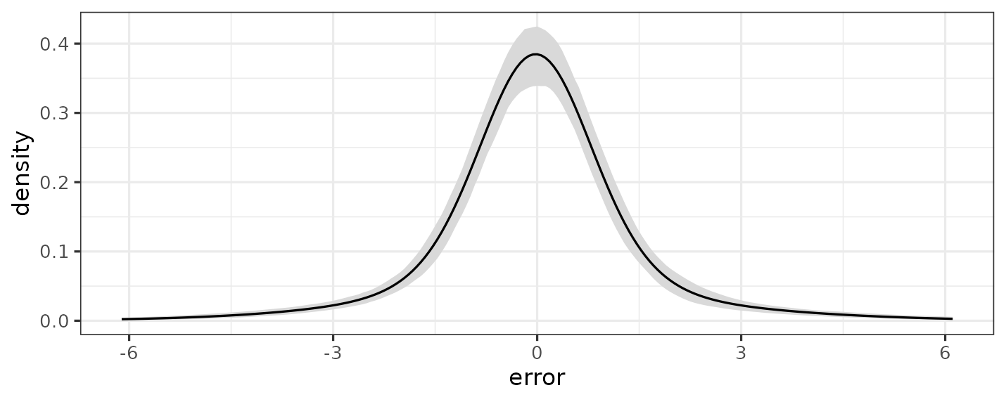

Positive Continuous Responses

The Gamma("log") family puts the forest on the log mean and draws the shape (i.e., the inverse dispersion), which is one value for the whole sample and so asserts that the coefficient of variation is constant. Gamma_ls() relaxes that: it gives the log dispersion a forest of its own, so the spread is free to move with the predictors the way gaussian_ls() lets a normal’s standard deviation move. Giving its second forest an intercept-only formula recovers the single-dispersion assumption, since ~ 1 names no predictor and leaves that forest a sum of stumps:

bartisan(y ~ x1 + x2, data = d, family = Gamma_ls())          # dispersion varies
bartisan(list(y ~ x1 + x2, ~ 1), data = d, family = Gamma_ls())  # and held constant

Write the link. stats::Gamma() defaults to link = "inverse", which is the canonical link for the gamma and the wrong one here: the additive predictor is unconstrained, and only the log link’s inverse keeps the mean positive over the whole line. A draw that wanders non-positive has no gamma density at all, so it is rejected during fitting and predict() returns NaN there. So bartisan ignores any other link and fits on "log", saying so once; writing Gamma("log") silences that. stats::Gamma() itself is untouched, so attaching the package cannot change what glm() does. If another link for a gamma response is genuinely wanted, custom_family() is the route. Gamma_ls() defaults to the log link without warning.

We compared Gamma(), Gamma_ls(), gaussian() with a "log" link, dpm(), and ordinal() with a probit link on 800 training and 800 test observations, 50 trees, 500 draws after 500 warmup, four replicates, over four shapes of error around one mean function, with each error centered so that \(E[Y \mid x]\) is the same function in every column. Gamma_ls() was given num_trees = c(50, 20). ordinal("probit") bins the outcome onto 25 quantiles and predicts with type = "mean", so its predictions are on the response’s scale even though its density is not, which is why it has no log score. Cells are RMSE / log score, medians over the replicates, and lower RMSE and higher log score are better.

Family	gamma, constant dispersion	gamma, varying dispersion	lognormal	heavy tail	seconds
Gamma("log")	0.395 / -1938	0.620 / -2218	0.548 / -2074	0.465 / -2097	7.6
Gamma_ls()	0.378 / -1940	0.461 / -2156	0.537 / -2073	0.440 / -2132	48.7
gaussian("log")	0.433 / -2096	1.265 / -2466	0.574 / -2366	1.229 / -2261	16.8
dpm()	0.793 / -2005	1.442 / -2251	0.913 / -2109	0.628 / -2042	2.4
ordinal("probit")	0.434	0.858	0.397	0.432	3.1

A few things to take from this:

Gamma_ls() is the family to reach for when the dispersion might vary, and it costs almost nothing when it does not. In the varying-dispersion column it cuts RMSE by 26% against Gamma("log") (0.461 against 0.620) and gains 62 log points. In the constant-dispersion column, where Gamma("log") is exactly right, the two are indistinguishable: 0.378 against 0.395 on RMSE and two log points apart, well inside the replicate-to-replicate spread. That is the same property that makes dpm() a safe default against gaussian(), and it is the argument for starting here when the outcome is positive and the spread is not known to be stable. What it costs is time, at about six times Gamma("log"), almost all of it in the dispersion forest, which takes the sampler’s general path where the mean forest does not.

ordinal("probit") on 25 bins has the best RMSE of any family in two of the four columns, on the lognormal error by 26% over Gamma_ls() and on the heavy tail by a hair, at a fraction of the cost and with no assumption about the error’s shape at all. What it gives up is the density on the original scale, and with it loo() comparisons against the other families here. It is the option to remember when the mean is the estimand and the error is a nuisance; see a continuous outcome as ordinal.

Binary Responses

The binomial() family accepts a 0/1 numeric response, a logical, a two-level factor, or a two-column matrix of successes and failures. For prediction, the link hardly matters ("logit" and "probit" differ by a scale factor of about 1.6 and give fitted probabilities that are hard to tell apart), so the choice is better made on grounds other than fit.

"logit" is the default because it is the default in stats::binomial(). Its predictor is a log odds, which is the scale many readers of a binary model expect, and it is the link under which a contrast has an odds-ratio reading.

"probit" reads the model as a normal latent variable crossing a threshold, which is the right link when that latent variable is the object of interest, and it is the one predict(type = "stdlv") is most natural for. It is also the fastest of the three.

"cloglog" is the one substantively different choice, because it is not symmetric: swapping the labels of success and failure gives a different model, where for logit and probit it gives the same model with the predictor negated. Use it when that asymmetry is the point: when the outcome is “at least one event occurred” and the underlying count is Poisson, where the complementary log-log model is exactly right, or in discrete time, where the cumulative version is the discrete proportional hazards model and the predictor is a log hazard ratio.

With very few events, the whole fit mixes slowly regardless of the link because a handful of events carry little information: at 2000 observations, the effective sample size of the level of the predictor fell from about 860 at half positives to 8 at 0.2%. Lengthen the chain and read diagnose().

Counts

The poisson() family restricts the conditional variance to equal the conditional mean, and the negbin() family adds a dispersion parameter reported as theta. The zi_poisson() and zi_negbin() families mix a point mass at zero (the zero-inflation part) with a count component and give each part its own forest (the first predictor is the log mean of the count, the second the log odds of being a structural zero), so the excess-zero mechanism can depend on the predictors. As with standard GLMs for count variables, these models can include an offset.

To decide which family to use, consider these two questions, in this order.

1. Are there more zeros than the count component can produce?

Not “are there many zeros”: a Poisson with a small mean produces plenty, and a forest can drive the mean low exactly where the zeros are. Fit the plain family and the zero-inflated one and compare with loo(). Reach for zero inflation when the zero mechanism is itself something to model, or when the two processes have different predictors, not merely to improve a fit.

It is worth seeing how far a marginal look at the response can mislead here. The counts below are Poisson with no inflation whatsoever, but the conditional mean ranges over two orders of magnitude, so the low end of it contributes a large pile of zeros:

set.seed(11)

nz <- 1000
dz <- data.frame(x1 = runif(nz), x2 = runif(nz), x3 = runif(nz))

# No zero inflation anywhere in this: one Poisson draw per observation
dz$count <- rpois(nz, exp(-3 + 5 * dz$x1 + 0.5 * dz$x2))

c(mean = mean(dz$count), zeros = mean(dz$count == 0),
  var_over_mean = var(dz$count) / mean(dz$count))
#>          mean         zeros var_over_mean 
#>          1.94          0.46          4.56

library(ggplot2)

ggplot(dz, aes(count)) +
  geom_histogram(binwidth = 1, fill = "grey70", colour = "white") +
  labs(x = "count", y = "observations",
       subtitle = "Poisson, no zero inflation, marginal mean 1.8") +
  theme_bw()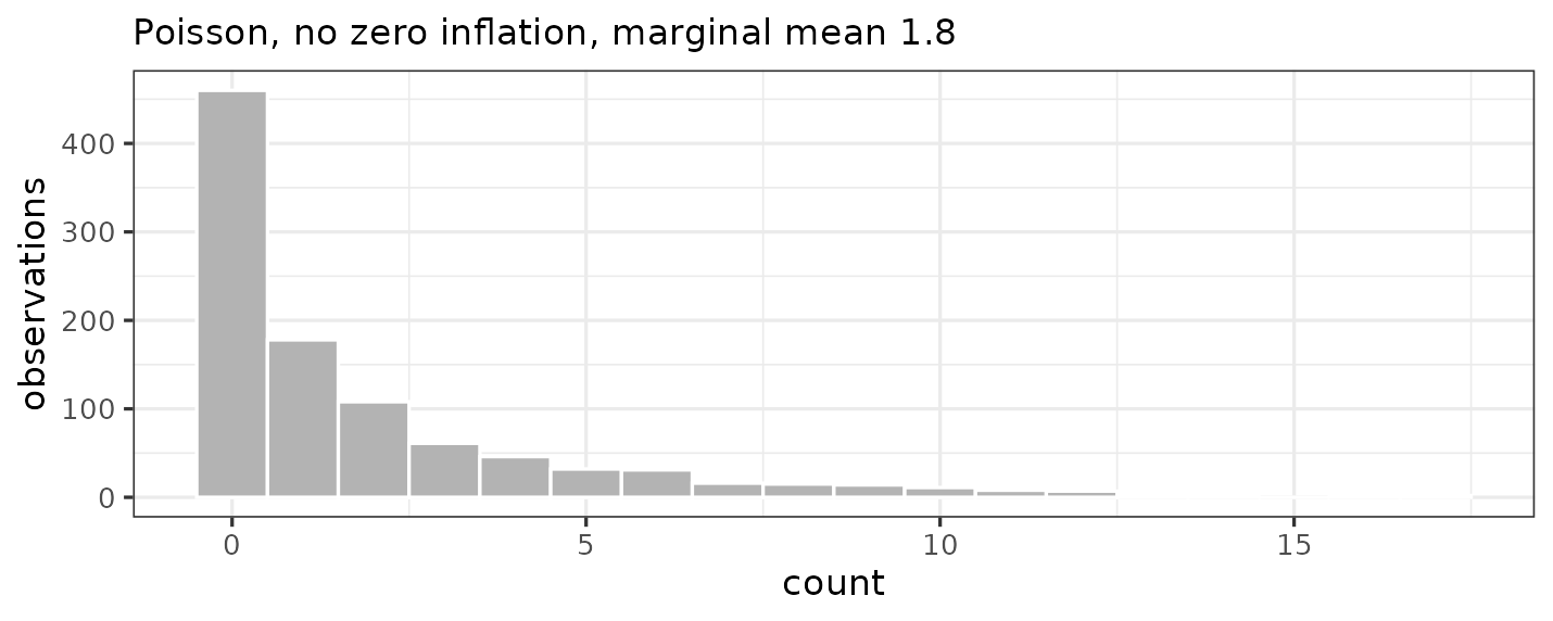

Nearly half the observations are zero, where a Poisson with the marginal mean of 1.9 would give 14%, and the variance is four and a half times the mean. On both of the marginal diagnostics usually reached for, these data look zero-inflated and overdispersed, and they are neither. Here the comparison uses fuller settings than the rest of this vignette, because a model comparison is what is being demonstrated and the small chains used elsewhere leave the differences inside their own standard errors:

count_control <- bartisan_control(num_trees = 50, num_burn = 500,
                                  num_draws = 500)

count_fit <- function(family) {
  set.seed(1)
  loo::loo(bartisan(count ~ x1 + x2 + x3, data = dz, family = family,
                    control = count_control))
}

loo::loo_compare(list(poisson = count_fit(poisson()),
                      negbin = count_fit(negbin()),
                      zi_poisson = count_fit(zi_poisson()),
                      zi_negbin = count_fit(zi_negbin())))
#>       model elpd_diff se_diff p_worse       diag_diff       diag_elpd
#>     poisson       0.0     0.0      NA                                
#>  zi_poisson      -1.3     0.7    0.97 |elpd_diff| < 4 1 k_psis > 0.63
#>   zi_negbin      -3.3     3.2    0.85 |elpd_diff| < 4 1 k_psis > 0.63
#>      negbin      -4.0     3.6    0.87 |elpd_diff| < 4
#> 
#> Diagnostic flags present.
#> See ?`loo-glossary` (sections `diag_diff` and `diag_elpd`)
#> or https://mc-stan.org/loo/reference/loo-glossary.html.

Read this the way vignette("comparison") recommends, which is to look at the standard errors before the ordering. Every difference here is within about two standard errors, so these data do not sharply separate any of the four, and that is worth saying before anything else. What they certainly do not do is prefer a zero-inflated fit: both zero-inflated families come out nominally behind the plain Poisson rather than ahead of it, despite a response that is 46% zeros, and zi_negbin(), which adds inflation and overdispersion at once, is nominally last. Since the truth here has neither, “no better than the plain Poisson” is the right answer rather than a failure to detect something.

What has happened is that the forest already accounts for the zeros by finding where the conditional mean is small, which is what a nonparametric mean is for, so a mixture has nothing left to explain and pays for its parameters. The lesson generalizes past counts: with a flexible mean, a feature of the marginal distribution of the response is not evidence about the conditional model. Reach for zero inflation when the zero mechanism is a process worth modeling in its own right, and let a comparison of fits, not a histogram, settle whether it is there.

2. Is the count component overdispersed once the zeros are accounted for?

A spike at zero inflates the sample variance and looks like dispersion. zi_negbin() separates the two at the cost of a parameter; if theta comes back large with a tight posterior, the negative binomial is not buying anything and zi_poisson() is the better-conditioned fit.

Once again, the ordinal() family is another option worth knowing about for counts. A count is ordered and takes few distinct values, which is exactly what the cutpoint structure is for: it makes no assumption about the count distribution, needs no dispersion parameter, and handles excess zeros without a mixture, since the zero category simply gets whatever probability the cutpoints give it. Predict with type = "mean" to get predictions on the original response scale. The limits are that it cannot predict a count larger than the largest one observed, and that it has no rate interpretation (i.e., no log link, so no incidence-rate ratio). It can be useful to bin first if the counts range over more than a few dozen values, as below.

Ordered Categories

The ordinal() family expects an ordered factor for the response variable, though a numeric response is accepted and its sorted unique values are taken as the categories. It uses the cumulative-link parameterization of MASS::polr() and WeightIt::ordinal_weightit(), in which \(P(Y \le k) = F(c_k - \eta)\), so larger values of the additive predictor shift mass toward higher categories.

Only the differences \(c_k - \eta_i\) are identified, so one location has to be pinned. With three or more categories, the draws are reported in the chart where the additive predictor has mean zero over the fitted sample and every cutpoint is free, which is what polr() and ordinal_weightit() report when its predictors are centered, and which makes the cutpoints readable as category boundaries. With exactly two categories, the single boundary is folded into the intercept instead, so a two-category response is exactly binary regression on the same scale¹.

The three links are read as for the binomial, plus one consideration specific to the ordinal case: the link decides what is held constant across categories. "logit" gives the proportional odds model, in which a contrast is a log odds ratio that is the same at every cutpoint. "probit" gives the ordered probit, and is the link to choose when the latent variable is the object of interest (e.g., a trait, a utility, an underlying measurement recorded in bins). "cloglog" gives the proportional hazards model on the categories, so choose it when the categories are ordered durations or stages. Accuracy is much the same across the three; "probit" is the fastest by a wide margin.

Ordered categories can also be treated as unordered categories and fit with family = multinomial(), described below; typically this produces more variable predictions as it requires a forest for each category rather than a single forest governing the entire distribution function.

A Continuous Outcome as Ordinal

ordinal() on a numeric response can be a useful way to model it, as demonstrated above. Every distinct value of \(Y\) becomes a category, the cutpoints absorb the marginal distribution of \(Y\), and the forest is left to explain only the ordering. Nothing is assumed about the error, and the model for \(P(Y \le y \mid x)\) is invariant to any monotone transformation of \(Y\) (i.e., fitting on \(Y\), \(\log Y\) or \(\sqrt Y\) gives the same model). This is the semiparametric ordinal regression rms::orm() fits for continuous outcomes, with a forest in place of the linear predictor. Predict with type = "mean", which reads the category labels as numbers and returns \(\sum_k y_{(k)} P(Y = y_{(k)} \mid x)\).

It can be useful to bin the outcome first in a smaller number of categories, as one cutpoint per distinct value means \(n\) cutpoints: at 1000 observations an unbinned fit took 73 seconds against 2.7 for gaussian(). Collapsing onto a grid of quantiles is both faster and more accurate, because a cutpoint vector with a thousand weakly-identified entries is worse conditioned than one with 25. Somewhere between 10 and 50 quantile bins is enough, and the choice inside that range hardly matters; 25 bins was sixteen times faster than no binning and slightly more accurate. Keep each bin’s mean as its label so that type = "mean" still reports on the outcome’s scale. See below for an example:

# Binning d$heavy
nbins <- 25

d$binned <- d$heavy |>
  quantile(seq(0, 1, length.out = nbins + 1)) |>
  unique() |>
  cut(x = d$heavy, include.lowest = TRUE, labels = FALSE) |>
  ave(x = d$heavy)

fit_oc <- bartisan(binned ~ x1 + x2,
                   data = d, control = ctrl,
                   family = ordinal("probit"))

head(predict(fit_oc, type = "mean"))
#> [1] 1.9576 2.4205 1.6156 2.1975 2.9249 0.0415

Two limits. type = "mean" is a convex combination of observed outcome values, so it can never predict outside the range of the training outcome, which is a feature when the outcome has a hard floor or ceiling and a liability when extrapolation is needed. And the invariance is a property of the model for \(P(Y \le y \mid x)\), not of the mean read off it: type = "mean" after fitting on \(\log Y\) is not the log of type = "mean" after fitting on \(Y\).

Unordered Categories

The multinomial() family expects an unordered factor. It can accept one of two links: "logit" and "probit". Start with link = "logit", the default: it is faster, its predictor is a log odds, and it is the parameterization most readers expect. By default it fits one forest per category and leaves the model unidentified (Murray 2021), which keeps the prior symmetric in the categories; every identified quantity is still recovered from the draws. Passing reference to multinomial() pins that category and fits one fewer forest, giving log odds against it the way nnet::multinom() and WeightIt::multinom_weightit() do, which may be a better choice when a particular contrast is the quantity of interest.

Choose link = "probit" when the alternatives are plausibly substitutes: it allows the latent utilities to be correlated, which a multinomial logit cannot express at all, so it is the link for when the independence-of-irrelevant-alternatives assumption is the one in doubt. Expect to pay in speed and in a simulated likelihood because the probabilities are Gaussian orthant probabilities with no closed form, so they and the reported log likelihood are computed by simulation.

With a multinomial probit family, the latent correlations are only weakly identified; we do not recommend reporting them as estimates. They enter the likelihood only through orthant probabilities of a distribution whose location is a sum of trees, and a flexible mean absorbs much of the dependence they are meant to capture. At 900 observations, the posterior tracked a swept true correlation only loosely and not monotonically, and the 95% intervals could cover more than half of the \((-1, 1)\) the parameter can occupy at all; repeating the zero case over eight draws of the data gave posterior means from \(-.60\) to \(.33\). By 3000 observations it behaves. What the probit link is still good for is the fit: allowing correlated errors changes the category probabilities whether or not \(\Sigma\) is pinned down.

Bounded Responses

The Beta() family is for beta regression with a response strictly inside the unit interval \((0, 1)\): a forest on the link of the mean \(\mu\) and a precision \(\phi\) drawn alongside it, so the response is distributed as \(\mathrm{Beta}(\mu\phi, (1-\mu)\phi)\) with variance \(\mu(1-\mu)/(1+\phi)\). The same three links as binomial() are allowed, read the same way.

d$rate <- rbeta(n, plogis(1.5 * sin(pi * d$x1)) * 12,
                12 - plogis(1.5 * sin(pi * d$x1)) * 12)

fit_beta <- bartisan(rate ~ x1 + x2, data = d, family = Beta(), control = ctrl)
mean(fit_beta$aux[, "phi"])
#> [1] 12.3

The ordbeta() family requests the ordered beta regression of Kubinec (2023), for a response on the closed unit interval \([0, 1]\) with point masses at zero and one (e.g., a percentage of a budget, a slider scale). One predictor drives both the probability of landing on an endpoint, through a pair of cutpoints as in an ordinal model, and the mean of the beta density in between.

Choose between Beta() and ordbeta() based on whether the response can reach a boundary, not on whether it happens to in the sample at hand. A response at zero or one has no beta density, so Beta() errors rather than nudging it inward. In the other direction, ordbeta() fitted to a response with no boundary observations leaves its two cutpoints with nothing to identify them; the fit is not much worse for it, but the cutpoints are not interpretable and drift to large magnitudes.

A Point Mass at Zero and a Continuous Positive Part

Spending, rainfall, insurance claims and earnings share a shape that none of the families above has: a genuine mass of exact zeros, and a skewed continuum above them. The tweedie() family is the compound Poisson–gamma, which models the pair as one process. A Poisson number of gamma-distributed amounts are added up, so a count of zero produces an exact zero and any positive count produces a positive amount, and the mean and variance come out as

\[\mathrm{E}[y \mid x] = \mu(x) = \exp(\eta(x)), \qquad \mathrm{Var}(y \mid x) = \phi\,\mu(x)^p\]

for a variance power \(p\) between 1 and 2. One forest does all of it, because the probability of a zero follows from the mean:

\[\Pr(y = 0 \mid x) = \exp\!\left(-\frac{\mu(x)^{2-p}}{\phi\,(2-p)}\right)\]

That tie is what makes this a single process rather than two, and it is also the assumption to check. The share of zeros has no level of its own: two people with the same mean have the same probability of a zero, with the functional form above. Where that is wrong, a two-part model is the alternative, and custom_family() is how to write one.

mu <- exp(1.5 + sin(pi * d$x1))
lambda <- mu^(2 - 1.5) / (4 * (2 - 1.5))
claims <- rpois(n, lambda)
d$spend <- ifelse(claims > 0,
                  rgamma(n, shape = claims * (2 - 1.5) / (1.5 - 1),
                         scale = 4 * (1.5 - 1) * mu^(1.5 - 1)),
                  0)

fit_tw <- bartisan(spend ~ x1 + x2, data = d, family = tweedie(), control = ctrl)
c(zeros = mean(d$spend == 0), phi = mean(fit_tw$aux[, "phi"]))
#> zeros   phi 
#> 0.213 3.743

The power argument is fixed at 1.5 by default rather than drawn, which is the one place this family differs from the rest in how its nuisance parameters are treated. The power is weakly identified at the sample sizes this package is used on, and a badly determined power drags the dispersion with it, since the two are identified jointly through the share of zeros. Pass power = NULL to draw it when the sample is large and the shape is of interest in itself; leave it alone when the mean is what is wanted.

Because the mean is \(\exp(\eta)\) and nothing more, a counterfactual mean needs nothing beyond the forest, and a tweedie() fit is directly comparable with a poisson() or Gamma("log") fit of the same response. A two-part model has no such property: its mean has to be recombined across two forests before anything can be contrasted.

Right-Censored Survival Times

There are five families that can be used with survival time response, all taking a survival::Surv() object. They differ in what the predictor means and in what the model leaves free:

Family	Model	A contrast in the predictor is	Left free
weibull_aft()	\(\log T = \eta + \sigma\epsilon\), \(\epsilon\) smallest extreme value	a log time ratio, and also a log hazard ratio	\(\sigma\)
loglogistic_aft()	the same with \(\epsilon\) logistic	a log time ratio	\(\sigma\)
lognormal_aft()	the same with \(\epsilon\) normal	a log time ratio	\(\sigma\)
dpm_aft()	\(\log T = \eta + W\), \(W\) a mixture	a log time ratio	the whole error density
ph()	\(\lambda(t \mid x) = \lambda_0(t)e^{r(x)}\)	a log hazard ratio	the baseline \(\lambda_0\)

All four accelerated failure time families share the structure \(\log T = \eta(x) + W\) with \(W\) independent of \(x\), and that alone makes a contrast in the predictor a log time ratio: every quantile of \(T\), its mean, and its geometric mean all scale by \(e^{\Delta\eta}\), whatever shape \(W\) has. What differs between them is what \(e^{\eta}\) is on its own, since each pins its error’s location differently, and vignette("survival") gives that per family. weibull_aft() is the only one whose predictor also carries a log hazard ratio, of \(-\Delta\eta/\sigma\), and that is a property of the smallest extreme value error rather than of the shared structure: it is the only error that makes an accelerated failure time model proportional hazards as well.

The three structured accelerated failure time families (i.e., the first three above) fix the shape of the error and so of the hazard, and are quick to fit. ph() frees the baseline hazard instead, so it fits a hazard of any shape, at the price of asserting proportionality and of reading the predictor on the hazard scale. dpm_aft() frees the error density (Henderson et al. 2020), which costs little when a single normal was right and gains a great deal when it was not.

dpm_aft() is the default for a Surv response, on the evidence in the survival vignette and because it is cheaper to fit than most of the alternatives. weibull_aft() is the one family that is both an accelerated failure time and a proportional hazards model, so it is the one to name when a hazard-ratio reading is what we want.

d$time <- rexp(n, exp(-(1 + d$x1)))
d$event <- rbinom(n, 1, 0.7)

fit_aft <- bartisan(survival::Surv(time, event) ~ x1 + x2,
                    data = d, control = ctrl,
                    family = weibull_aft())

colMeans(fit_aft$aux)
#> sigma 
#>  1.03

The survival function comes from predict(., type = "survival"), which takes the times to report it at and works for every family in the table:

fit_ph <- bartisan(survival::Surv(time, event) ~ x1 + x2,
                   data = d, control = ctrl,
                   family = ph())

head(predict(fit_ph, type = "survival", times = c(1, 2, 5)), 3)
#>          1     2     5
#> [1,] 0.867 0.758 0.524
#> [2,] 0.853 0.734 0.485
#> [3,] 0.802 0.653 0.369

It is also the estimand we usually want. The question is rarely about the predictor but about survival at a horizon (e.g., the difference in one-year survival between two groups), and that is a contrast of type = "survival" at one time.

We recommend dpm_aft() as the default when we have no view about the shape of anything; measured against five alternatives over six data-generating truths, it was best or tied-best on four and never worse than third, and it matched the correctly specified family on the two truths where one existed. Use lognormal_aft() or loglogistic_aft() when the fit has to be quick, weibull_aft() when a hazard-ratio reading is wanted from a parametric fit, and ph() when the shape of the baseline hazard is the point. If the covariate effect may move with time, so that survival curves cross, none of the five is right and the discrete-time route is.

The trade-offs behind these choices are measured in vignette("survival", package = "bartisan"), which covers what each estimand is, which hazard shapes each family can and cannot represent, how they behave under censoring and under misspecification, the discrete-time route for non-proportional hazards, and one trap in comparing their log scores.

Other Links and Custom Likelihoods

Links beyond those in the table are accepted for gaussian(), binomial(), poisson(), negbin() and Beta(), and applied from R by composing the supplied inverse link with the family’s own. So binomial("cauchit") works, as does any link object of the kind stats::make.link() returns, including one written by hand. Two cautions: 1) the fit is slower, because each leaf costs a call into R, and 2) the additive predictor is unconstrained, so a link whose inverse has a restricted range (e.g., poisson("identity")) gives non-finite densities for some predictors, which are rejected rather than breaking the chain but are wasted work. bartisan() reports that when the fit starts. The families with more than one predictor, or whose link enters somewhere other than a single mean, take only their listed links.

custom_family()can be used to fit a BART model with a density of the user’s design. It takes the log density itself and fits the model that goes with it. The sampler needs only the first two derivatives with respect to each additive predictor, and central differences of the supplied function produce both. Terms free of eta, the predictor to be modeled by BART, may be dropped: they cancel from every acceptance ratio. See below for an example of a “hand-rolled” Poisson fit using the Poisson density dpois().

# Custom Poisson family
pois_by_hand <- custom_family(
  logdens = function(y, eta) dpois(y, exp(eta[, 1]), log = TRUE),
  start   = log(mean(d$count)),
  name    = "hand-rolled Poisson")

fit_custom <- bartisan(count ~ x1 + x2,
                       data = d, control = ctrl,
                       family = pois_by_hand)

# Internal Poisson family
fit_pois <- bartisan(count ~ x1 + x2,
                     data = d, control = ctrl,
                     family = poisson())

cor(predict(fit_custom, type = "link"),
    predict(fit_pois, type = "link"))
#> [1] 0.998

The function is called once per leaf per Fisher-scoring step with the observations reaching that leaf, so it must be vectorized over y and the rows of eta and must return exactly one value per row. Ask for several additive predictors with num_predictors; supply derivatives when they are easy to write down, which cuts three calls to one and removes the differencing error. See ?custom_family for details.

Nuisance parameters are drawn too, if they are named. logdens then takes a third argument holding their current values, and the draws come back in fit$aux under the names given, covered by summary() and diagnose() like any other family’s:

# Custom Gaussian family
gauss_by_hand <- custom_family(
  logdens   = function(y, eta, aux) dnorm(y, eta[, 1], exp(aux[1]), log = TRUE),
  aux_start = c(log_sigma = 0),
  start     = mean(d$heavy))

fit_aux <- bartisan(heavy ~ x1 + x2,
                    data = d, control = ctrl,
                    family = gauss_by_hand)

# Internal Gaussian family
fit_gauss <- bartisan(heavy ~ x1 + x2,
                      data = d, control = ctrl,
                      family = gaussian())

cor(predict(fit_aux, type = "link"),
    predict(fit_gauss, type = "link"))
#> [1] 0.974

# Estimate of the auxiliary parameter
summary(exp(fit_aux$aux[, "log_sigma"]))
#>    Min. 1st Qu.  Median    Mean 3rd Qu.    Max. 
#>    1.43    1.55    1.59    1.59    1.63    1.78
summary(fit_gauss$aux[, "sigma"])
#>    Min. 1st Qu.  Median    Mean 3rd Qu.    Max. 
#>    1.41    1.55    1.59    1.60    1.64    1.76

There is no prior argument and no bounds argument. A parameter with a restricted range is handled the way it would be for a real predictor, by writing the transform into logdens, which is what the exp(aux[1]) above is doing. aux_start need only be the right order of magnitude; the sampler walks to the posterior from a poor start.

What it cannot do: take a non-numeric response, so a factor has to be coded first; or report a fitted mean, since the package cannot know what the mean of a supplied density is, so predict(type = "response") returns the additive predictors instead, though type = "density" works.

Custom likelihoods are why bartisan is named what it is; they support artisanal models augmented by BART. Anywhere you might otherwise include a linear predictor in a model, it can be estimated flexibly with BART instead.

References

George, Edward, Purushottam Laud, Brent Logan, Robert McCulloch, and Rodney Sparapani. 2019. “Fully Nonparametric Bayesian Additive Regression Trees.” In Topics in Identification, Limited Dependent Variables, Partial Observability, Experimentation, and Flexible Modeling: Part b, vol. 40B. Advances in Econometrics. Emerald Publishing Limited. https://doi.org/10.1108/S0731-90532019000040B006.

Henderson, Nicholas C., Thomas A. Louis, Gary L. Rosner, and Ravi Varadhan. 2020. “Individualized Treatment Effects with Censored Data via Fully Nonparametric Bayesian Accelerated Failure Time Models.” Biostatistics 21 (1): 50–68. https://doi.org/10.1093/biostatistics/kxy028.

Kubinec, Robert. 2023. “Ordered Beta Regression: A Parsimonious, Well-Fitting Model for Continuous Data with Lower and Upper Bounds.” Political Analysis 31 (4): 519–36. https://doi.org/10.1017/pan.2022.20.

Linero, Antonio R. 2025. “Generalized Bayesian Additive Regression Trees Models: Beyond Conditional Conjugacy.” Journal of the American Statistical Association 120 (549): 356–69. https://doi.org/10.1080/01621459.2024.2337156.

Murray, Jared S. 2021. “Log-Linear Bayesian Additive Regression Trees for Multinomial Logistic and Count Regression Models.” Journal of the American Statistical Association 116 (534): 756–69. https://doi.org/10.1080/01621459.2020.1813587.