Reports, for every predictor, how many splitting rules the forest spends on
it and how often it is used at all, which is what "variable importance" means
for a BART model. This is the table summary.bartisan_fit() prints, returned
as a data frame rather than displayed (i.e., ready to sort, filter, or plot).
Usage
variable_importance(object, level = 0.95, draws = FALSE, plot = FALSE)

# S3 method for class 'bartisan_importance'
plot(x, y, ...)
Arguments
- object
a
<bartisan_fit>object; the output of a call tobartisan().- level
numeric; the width of the interval reported forsplits. Default is .95 for a 95% interval.- draws
logical; whether to return the splitting counts of every posterior draw rather than a summary of them, which is what to use for a comparison the summary does not offer (e.g., the posterior probability that one predictor takes more rules than another). Default isFALSEto return the summary. Cannot be combined withplot.- plot
logical; whether to return a plot of the table instead of the table, as a ggplot2 object showingsplitsand its interval for each predictor. Default isFALSE. Equivalent to callingplot()on the result, which is usually the more convenient of the two since the table can be subset first (e.g.,plot(head(imp, 10))for a wide model). ggplot2 must be installed for either.- x
a
<bartisan_importance>object; the output of a call tovariable_importance().- y
not used.
- ...
not used.
Value
A <bartisan_importance> object, which is a data frame with one row per
predictor and its own print() and plot() methods, sorted by prop_used
and then
splits, both decreasing, and with the following columns:
variable: the predictor, under the name the formula gave itprop_used: the proportion of draws in which it received at least one ruleprop_splits: its share of all the splitting rules in the forest, averaged over drawssplits: the mean number of splitting rules per draw that use itsplits_lowerandsplits_upper: the endpoints of thelevelinterval on that number, which theprint()method leaves out of the displayed table
A family with more than one additive predictor has a forest for each, and the
data frame then gains a leading predictor column naming which.
With draws = TRUE, the draws-by-predictors matrix of counts instead, or a
named list of them when there is more than one forest. With plot = TRUE, a
ggplot2 object.
Details
Which Column Answers Which Question
prop_used (the proportion of posterior draws in which the predictor
received at least one splitting rule) is the one to read first. It behaves
like a posterior probability that the predictor belongs in the model, and it
separates signal from noise sharply once sparsity = TRUE in
bartisan_control(), which puts a Dirichlet prior on how the rules are shared
out and lets unused predictors be dropped rather than merely used rarely. With
sparsity = FALSE every predictor keeps a share of the rules and prop_used
sits near 1 throughout, so the print() method says so rather than leaving
the column to be misread.
prop_splits is the one to reach for when two fits are being compared.
splits counts rules, so it scales with num_trees and a fit of 40 trees
will report four times the count of a fit of 10 without being four times as
informative; the share is computed within each draw before averaging, so the
shares add to one whatever the forest size. Note that the share is a property
of the forest and not only of the predictor, so it can still shift when the
forest size changes how the rules are allocated; the ranking is the stable
part.
splits, the mean number of rules per draw, says how much of the forest's
structure a predictor accounts for. It is the more familiar number and the
easier one to over-read.
Three Things This Is Not
It is not an effect size. A predictor can be split on constantly and move
the prediction very little, and the reverse happens too. If the question is
how much a predictor moves the outcome, that is a job for
marginaleffects::avg_comparisons()
on the fitted model, not for this
table. See bartisan-marginaleffects.
It is not stable under correlated predictors. When two predictors carry
the same information the trees split on whichever is convenient, and the usage
distributes between them more or less arbitrarily. A predictor can matter and
still show a low prop_used because a collinear partner absorbed it, so a
group of correlated predictors is best read as a group.
It is not causal. A ranking of predictors by usage is a description of this fitted function, not of what would happen if any of them were changed.
Reading It as Variable Selection
With sparsity = TRUE, prop_used is usable as a selection rule: predictors
the forest genuinely needs sit near 1 and the rest fall near 0, usually with a
wide gap rather than a continuum. It is the posterior inclusion probability
that the Dirichlet prior was introduced to make readable (Linero, 2018), and
cutting it at .5 gives the median probability model, which Barbieri and Berger
(2004) show is often a better predictive submodel under squared error loss
than the model of highest posterior probability. That is the same quantity and
the same cut SoftBart reports from a soft BART fit, computed from the
same splitting counts. No threshold is correct in general, though, so the gap
is the thing to look at, and a conclusion worth reporting will not depend on
where in it the cut is made.
The .5 cut chooses a predictive submodel and is not a test, and it does not
behave like one. On data where no predictor matters at all, at \(n = 300\)
with 25 predictors and 20 trees, it selected 7 of the 25 on average with
sparsity = TRUE and all 25 with sparsity = FALSE. A forest asked to fit
noise still puts its rules somewhere, and prop_used reports where they went
rather than whether they were needed.
References
Barbieri, M. M., & Berger, J. O. (2004). Optimal predictive model selection. The Annals of Statistics, 32(3). doi:10.1214/009053604000000238
Bleich, J., Kapelner, A., George, E. I., & Jensen, S. T. (2014). Variable selection for BART: an application to gene regulation. The Annals of Applied Statistics, 8(3). doi:10.1214/14-AOAS755
Linero, A. R. (2018). Bayesian regression trees for high-dimensional prediction and variable selection. Journal of the American Statistical Association, 113(522), 626–636. doi:10.1080/01621459.2016.1264957
See also
summary.bartisan_fit(), which prints the same table;
bartisan_control() for sparsity; bartisan-marginaleffects for effects
rather than usage
Examples
data("rhc")
set.seed(123)

# The sparsity prior concentrates the splitting rules on the predictors that
# earn them, which is what makes `prop_used` readable as a selection rule
fit <- bartisan(death ~ . - days, data = rhc, num_trees = 10,
                num_burn = 50, num_draws = 50, sparsity = TRUE,
                verbose = FALSE)
#> ℹ Using `family = binomial()`.
#> ℹ Set `family` to choose another, which also silences this message.

imp <- variable_importance(fit)
imp
#> Variable importance
#>
#>  variable prop_used prop_splits splits
#>     paco2      1.00       0.207    3.0
#>    surv2m      1.00       0.170    2.5
#>       age      1.00       0.104    1.5
#>       aps      0.96       0.135    2.0
#>      card      0.76       0.054    0.8
#>       rhc      0.64       0.083    1.3
#>      pafi      0.58       0.093    1.4
#>      resp      0.44       0.035    0.5
#>      crea      0.42       0.039    0.5
#>      race      0.20       0.052    0.8
#>       edu      0.18       0.012    0.2
#>    meanbp      0.12       0.010    0.2
#>      hema      0.06       0.004    0.1
#>       sex      0.02       0.002    0.0
#>
#> ℹ splits_lower and splits_upper hold the 95% interval, not shown above.

# The predictors the forest reaches for in nearly every draw
subset(imp, prop_used > .9)
#> Variable importance
#>
#>  variable prop_used prop_splits splits
#>     paco2      1.00       0.207    3.0
#>    surv2m      1.00       0.170    2.5
#>       age      1.00       0.104    1.5
#>       aps      0.96       0.135    2.0
#>

# `prop_splits` is the column that survives a change of forest size, since
# the shares add to one however many rules there are to share
big <- bartisan(death ~ . - days, data = rhc, num_trees = 40,
                num_burn = 50, num_draws = 50, sparsity = TRUE,
                verbose = FALSE)
#> ℹ Using `family = binomial()`.
#> ℹ Set `family` to choose another, which also silences this message.

merge(variable_importance(fit)[c("variable", "prop_splits")],
      variable_importance(big)[c("variable", "prop_splits")],
      by = "variable", suffixes = c("_10", "_40"))
#>    variable prop_splits_10 prop_splits_40
#> 1       age    0.103936407     0.10915611
#> 2       aps    0.135239912     0.07412900
#> 3      card    0.053880291     0.04540793
#> 4      crea    0.038787046     0.03804600
#> 5       edu    0.011627631     0.04547107
#> 6      hema    0.004250000     0.05491165
#> 7    meanbp    0.010388655     0.05604351
#> 8     paco2    0.206618692     0.07269543
#> 9      pafi    0.093291556     0.09744325
#> 10     race    0.052406593     0.07787674
#> 11     resp    0.035172308     0.03435895
#> 12      rhc    0.082606194     0.06000012
#> 13      sex    0.001538462     0.07148764
#> 14   surv2m    0.170256252     0.16297259

# The counts themselves, for a comparison the summary does not make
counts <- variable_importance(fit, draws = TRUE)
mean(counts[, "aps"] > counts[, "meanbp"])
#> [1] 0.86

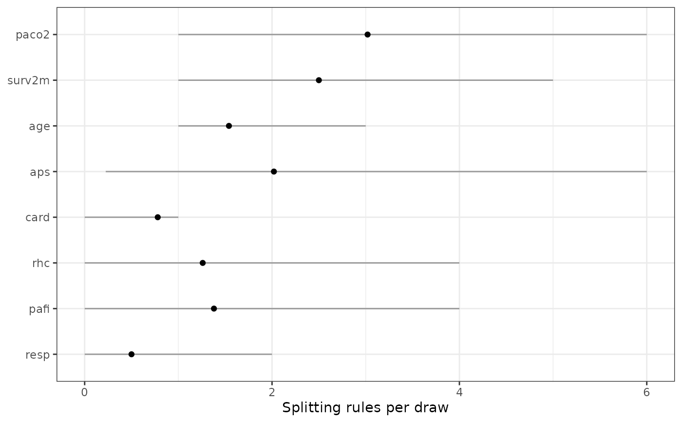
# The ranking, drawn. Subsetting first is what keeps a wide model readable.
plot(head(imp, 8))