Error distribution of a Dirichlet process mixture fit

Estimates the density of the errors of a dpm() or dpm_aft() fit, as the posterior of the density of a new error evaluated on a grid. Where BART commits to one normal, this says what shape the errors actually have.

Usage

error_density(object, at = NULL, level = 0.95, plot = FALSE, iterations = NULL)

# S3 method for class 'bartisan_error_density'
plot(x, y, ...)

Arguments

object

a <bartisan_fit> object fit with family = dpm() or family = dpm_aft(); every other family fixes the error distribution, so its density is a closed form rather than something to estimate.

at

numeric; the grid to evaluate the density on. Default is NULL for 201 points spanning four posterior-mean error standard deviations either side of zero.

level

numeric; the width of the pointwise interval. Default is .95 for 95% intervals.

plot

logical; whether to return a plot of the density rather than the density itself. Default is FALSE to return the values. Equivalent to calling plot() on the result. Either needs ggplot2 and returns a ggplot object, so it can be added to in the usual way; the values are the thing to reach for when the density is to be drawn against something else, as vignette("survival") draws it against the normal a lognormal_aft() fit would have assumed.

iterations

numeric; optional indices of the stored draws to use, between 1 and the number of draws the fit retains. Default is NULL to use all of them.

x

a <bartisan_error_density> object; the output of a call to error_density().

y

not used.

...

ignored; present for compatibility with the generic.

Value

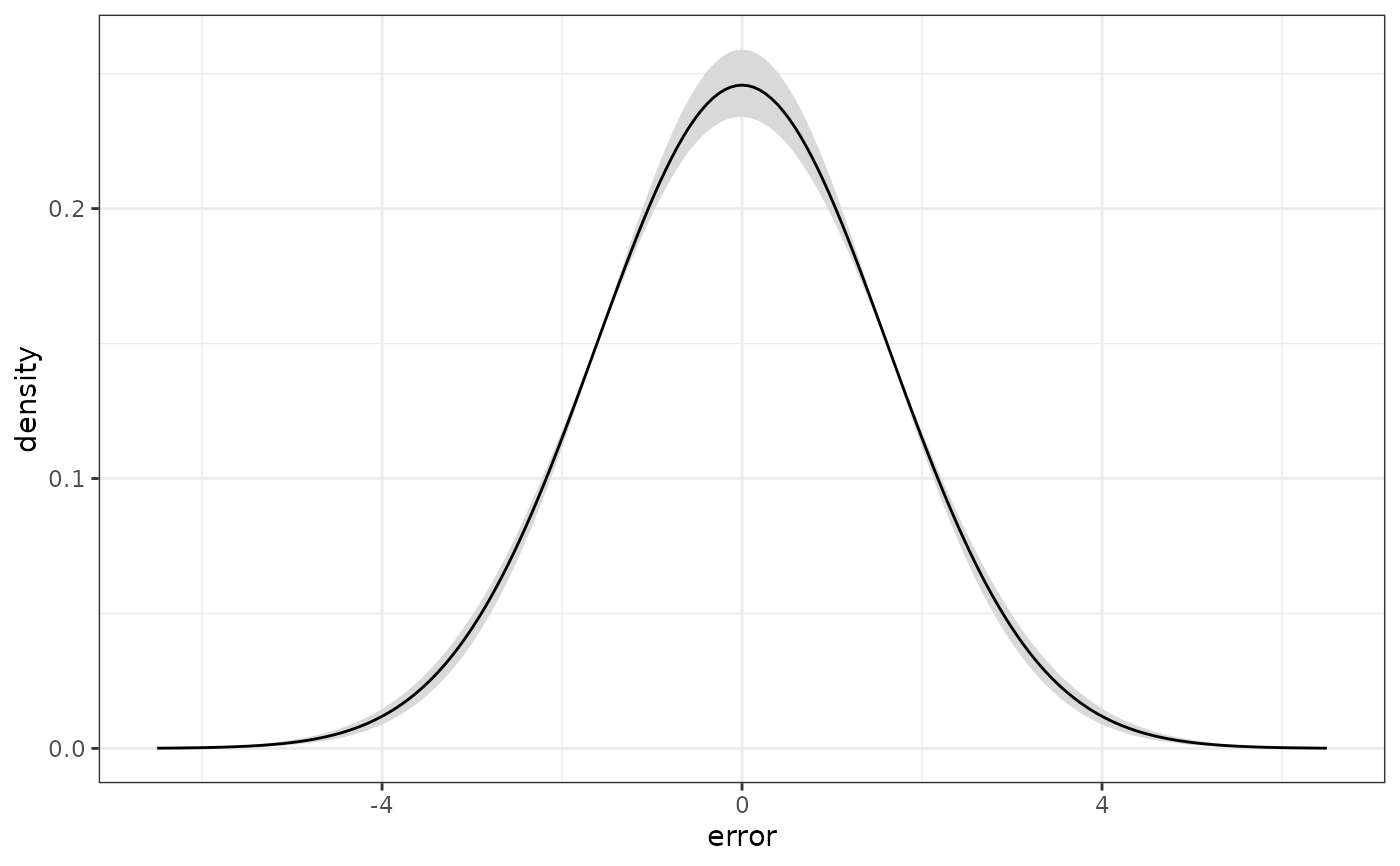
A <bartisan_error_density> object, which is a data frame with one row per grid point and its own plot() method, with columns at, mean, lower, and upper, giving the posterior mean density and a pointwise interval. With plot = TRUE, or from plot() on the result, a ggplot object drawing the posterior mean density with that interval as a ribbon.

See also

dpm() and dpm_aft() for the families with an estimated error distribution; bartisan()

Examples

data("rhc")
set.seed(123)

# How long a patient survived, among those who died, so that the outcome is
# a complete rather than a censored time
died <- rhc[rhc$death == 1, ]
died$log_days <- log(died$days)

fit <- bartisan(log_days ~ . - death - days, data = died, family = dpm(),
                num_trees = 10, num_burn = 50, num_draws = 50)

# What shape the errors have, which is what a Gaussian fit would have
# assumed to be normal
head(error_density(fit, at = c(-2, 0, 2)))
#>   at      mean     lower     upper
#> 1 -2 0.1149753 0.1115021 0.1177285
#> 2  0 0.2457427 0.2339895 0.2589215
#> 3  2 0.1149345 0.1115033 0.1173836

# The same thing drawn, with the pointwise interval as a ribbon
plot(error_density(fit))