Methods for Bayesian causal forest fits

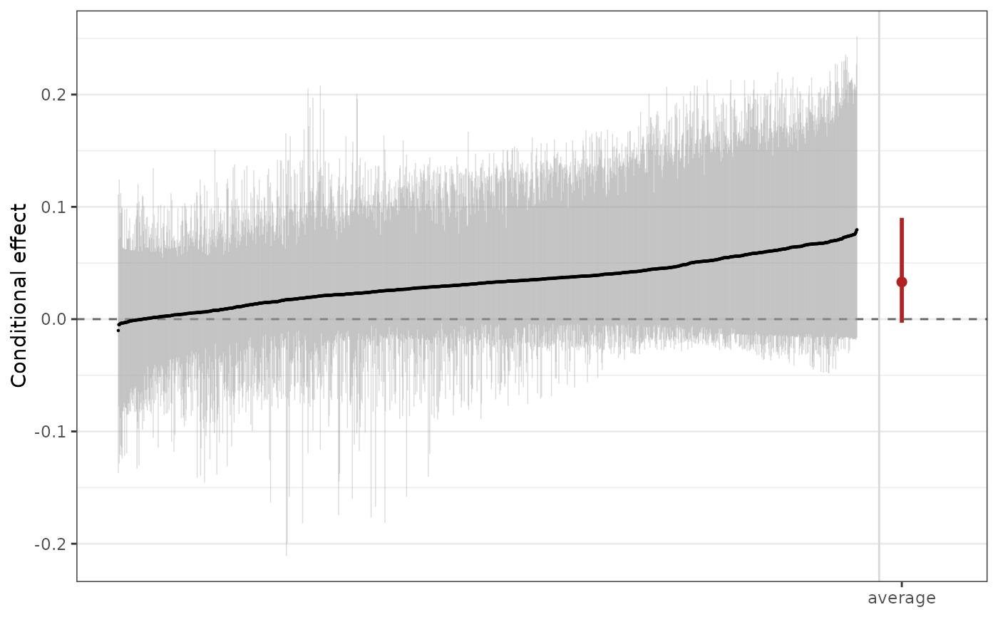
A fit from bcf() is a <bartisan_fit> with a treatment named, so it takes every method that fit takes. print() adds the treatment and says where the effect comes from, and plot() draws the conditional effects.

Usage

# S3 method for class 'bcf_fit'
print(x, digits = 3L, ...)

# S3 method for class 'bcf_fit'
plot(x, level = 0.95, comparison = "difference", ...)

Arguments

x

a <bcf_fit> object; the output of a call to bcf().

digits

integer; the number of significant digits to print.

...

for plot(), further arguments passed to estimate_effect(); otherwise ignored.

level

numeric; the level of the credible interval. Default is .95.

comparison

passed to estimate_effect(), which is what computes the numbers.

Value

plot() returns a ggplot2 object. print() returns its input invisibly.

Details

The effect itself is estimate_effect()'s to report, and summary() on a <bcf_fit> is the same summary of the forests it is on any other fit, with a line at the end saying so. That way the same call prints the same thing whether the model came from bcf() or from bartisan() with a vc() term.

See also

estimate_effect() for the effect and its estimands; bcf() for the model

Examples

data("rhc")
set.seed(123)

fit <- bcf(death ~ age + sex + meanbp + aps, treat = ~ rhc,
           data = rhc, num_trees = 10, num_burn = 50, num_draws = 50,
           verbose = FALSE)
#> ℹ Using `family = binomial()`.
#> ℹ Set `family` to choose another, which also silences this message.

fit
#> Generalized BART
#> 
#> Call:
#> bcf(formula = death ~ age + sex + meanbp + aps, treat = ~rhc, 
#>     data = rhc, num_trees = 10, num_burn = 50, num_draws = 50, 
#>     verbose = FALSE)
#> 
#> Family: "binomial" with the "logit" link
#> Observations: 1500
#> Structure: 2 forests of 10 trees, soft decision rules
#> Draws: 50 kept after 50 warmup
#> 
#> Posterior means: b.rhc.0 = 0.239, b.rhc.1 = 0.455
#> 
#> Treatment: "rhc"
#> Effect moderators: "age", "sex", "meanbp", and "aps"
#> ℹ `estimate_effect()` reports the treatment effect, with the average potential
#>   outcomes beside it; `plot()` draws the conditional ones.

# The effect, with the potential outcomes it is a difference of
estimate_effect(fit)
#> Average treatment effect (difference)
#> 
#> Treatment: "rhc"
#> Averaged over 1500 units
#> 
#>     contrast estimate    lower  upper    n
#>  Y[1] - Y[0]   0.0331 -0.00319 0.0902 1500
#> 
#> Average potential outcomes
#> 
#>  quantity estimate lower upper
#>      Y[0]    0.642 0.615  0.67
#>      Y[1]    0.675 0.647  0.71
#> 
#> ℹ estimate is the posterior mean; lower and upper bound the 95% equal-tailed
#>   credible interval.
#> ℹ Y[a] is the average response with "rhc" set to a.

# The conditional effects, ordered, with the average beside them
plot(fit)