Causal effects from a fitted model

Estimates the average or conditional effect of a treatment by g-computation over the posterior draws. estimate_effect() predicts every unit under every level of the treatment, contrasts those potential outcomes within each draw, and averages over the units the estimand asks for.

Usage

estimate_effect(
  object,
  treat = NULL,
  estimand = "ATE",
  comparison = "difference",
  by = NULL,
  newdata = NULL,
  level = 0.95,
  interval = "eti",
  focal = NULL,
  type = "response",
  plot = FALSE
)

# S3 method for class 'bartisan_effect'
print(x, digits = 3L, contrasts = NULL, potential_outcomes = TRUE, ...)

# S3 method for class 'bartisan_effect'
plot(x, ...)

Arguments

object: a <bartisan_fit> object; the output of a call to bcf() or bartisan().
treat: string; the name of the treatment variable. A fit from bcf() carries its own and needs none, so this is for a fit from bartisan(), where nothing marks one predictor as the treatment.
estimand: string; which units the effect is averaged over. "ATE" (the default) uses all of them, and "ATT" and "ATC" those in the focal group, which by default is the treatment's second level for the former and its first for the latter. With a binary treatment that makes them the treated and the untreated without focal being named. "CATE" does not average at all and returns one effect per unit. Abbreviations and lowercase spellings are allowed.
comparison: string; how the two potential outcomes are contrasted. Allowable options include "difference" (the default), "ratio", "lnratio", "or", and "lnor". The last two are available only when the response is a probability.
by: optional; a one-sided formula or a variable name naming a grouping variable, in which case the effect is averaged within each of its levels rather than over the whole sample.
newdata: optional; a data frame of units to average over. Default is the data the model was fit to, which is what makes the default estimand the sample average effect.
level: numeric; the level of the credible interval. Default is .95.
interval: string; "eti" (the default) for an equal-tailed interval from the quantiles of the draws, or "hpdi" for the highest posterior density interval, which is the shortest interval containing level of the posterior mass.
focal: optional; the treatment level whose units the effect is averaged over for "ATT" and "ATC". With a binary treatment it defaults to the second level for "ATT" and the first for "ATC", which makes them the effect among the treated and among the untreated. With a treatment of more than two levels it has no default and must be supplied, and then "ATT" and "ATC" differ only in the level named.
type: string; the prediction scale the effect is computed on, passed to predict.bartisan_fit(). Default is "response", which is the scale on which an average of unit-level differences is the marginal effect. See Details before changing it.
plot: logical; whether to draw the result rather than return it. Default is FALSE. plot = TRUE calls plot.bartisan_effect().
x: a <bartisan_effect> object; the output of a call to estimate_effect().
digits: integer; the number of significant digits to print.
contrasts: string; which contrasts to display when the treatment has more than two levels. "focal" (the default when a focal group is known) shows only the contrasts involving it, "all" shows every pairwise contrast, and a character vector of contrast labels shows those. All of them are computed either way; this only decides what is printed.
potential_outcomes: logical; whether to print the average response under each treatment level below the contrasts, those being what the contrasts were computed from. Default is TRUE. They are in the result's "potential_outcomes" attribute either way.
...: ignored.

Value

A <bartisan_effect> object, a data frame with one row per reported effect and columns contrast, estimate, lower, and upper, plus unit when estimand = "CATE" and the by variable's name when by is used. The posterior draws of every reported quantity are kept in the "draws" attribute, and the marginal mean of each potential outcome in "potential_outcomes", so a caller can re-contrast or re-summarize without refitting.

print() returns its input invisibly, and prints the potential outcomes below the contrasts unless potential_outcomes = FALSE. plot() returns a ggplot2 object.

Details

Why the Response Scale

A varying coefficient is a contrast on the link scale: on a binomial("logit") fit, coef(object) is a per-unit difference in log odds. The average of those is the average conditional log odds ratio, which is not the marginal log odds ratio and is not usually the quantity a treatment question asks for. So the default here is type = "response", where every unit's contrast is on the scale the response is measured on and averaging them is the marginal effect.

type = "link" is still available and is the right choice for looking at how the effect varies, since that is the scale the forest models it on. It is the wrong choice for reporting an average.

Marginal Rather Than Average Conditional

For "ratio", "lnratio", "or" and "lnor" the potential outcomes are averaged over units first and contrasted afterward, which gives the marginal ratio. With estimand = "CATE" there is no averaging to do, so a ratio reported there is a conditional ratio and the print() method says so.

For the same reason "or" and "lnor" are not each other's exp() and log(). Each summarizes the posterior of the quantity it names, and a posterior mean does not survive a nonlinear transformation: "or" reports the mean of the odds ratio and "lnor" the mean of its logarithm, which exponentiates to something smaller. Report whichever scale the interval should be symmetric on, which for a ratio is usually the log. The same holds of "ratio" against "lnratio".

Which Level Is Treated

With a binary treatment and no focal, which level is the treated one is worked out from the treatment's values by the rules WeightIt::weightit() uses, so that the same variable is read the same way by both packages. In order: a logical treatment is treated at TRUE; a numeric one is untreated at 0; a character or factor one whose levels parse as numbers is untreated at 0, or else treated at the largest; and otherwise the conventional names are matched, "t", "tr", "treat", "treated" and "exposed" against "c", "co", "ctrl", "control" and "unexposed". When none of those applies the second level is taken as the treated one and a message says so, that being the case where the guess can be wrong. "ATC" takes the other level as its focal group, so both estimands average over the group focal names and only the default differs.

Multi-category Treatments

There is nothing to work out from the values, so focal is required for "ATT" and "ATC", and those two then name the same estimand: the effect among the units in the level named.

Every pairwise contrast is computed. Which ones are shown is a display choice, made by contrasts in the print() method: with a focal group the default is to show only the contrasts involving it, matching how WeightIt::weightit() and cobalt::bal.tab() use focal.

A continuous treatment is not currently supported, because the effect of a continuous treatment is a slope or a dose-response curve rather than a contrast of levels. See the adrftools package for tools to visualize and summarize the effect of a continuous treatment.

Examples

data("rhc")
set.seed(123)

fit <- bcf(death ~ age + sex + meanbp + aps, treat = ~ rhc,
           data = rhc, num_trees = 10, num_burn = 50, num_draws = 50,
           verbose = FALSE)
#> ℹ Using `family = binomial()`.
#> ℹ Set `family` to choose another, which also silences this message.

# The risk difference, averaged over everyone
estimate_effect(fit)
#> Average treatment effect (difference)
#> 
#> Treatment: "rhc"
#> Averaged over 1500 units
#> 
#>     contrast estimate    lower  upper    n
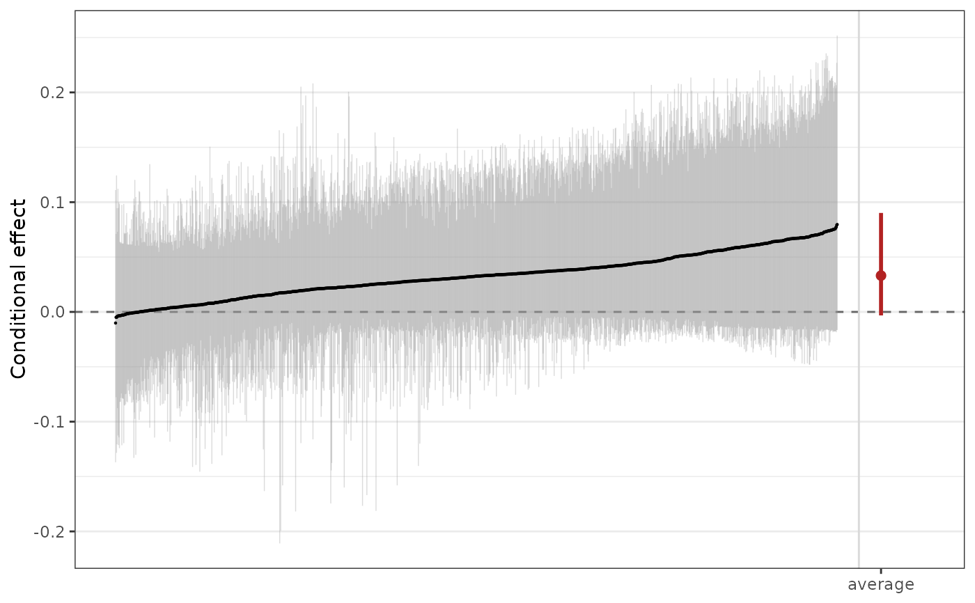
#>  Y[1] - Y[0]   0.0331 -0.00319 0.0902 1500
#> 
#> Average potential outcomes
#> 
#>  quantity estimate lower upper
#>      Y[0]    0.642 0.615  0.67
#>      Y[1]    0.675 0.647  0.71
#> 
#> ℹ estimate is the posterior mean; lower and upper bound the 95% equal-tailed
#>   credible interval.
#> ℹ Y[a] is the average response with "rhc" set to a.

# Among the treated, and as a risk ratio rather than a difference
estimate_effect(fit, estimand = "ATT", comparison = "ratio")
#> Average treatment effect on the treated (ratio)
#> 
#> Treatment: "rhc"
#> Averaged over the 565 units in group "1"
#> 
#>     contrast estimate lower upper   n
#>  Y[1] / Y[0]     1.04 0.996  1.13 565
#> 
#> Average potential outcomes
#> 
#>  quantity estimate lower upper
#>      Y[0]    0.668 0.633 0.701
#>      Y[1]    0.696 0.668 0.728
#> 
#> ℹ estimate is the posterior mean; lower and upper bound the 95% equal-tailed
#>   credible interval.
#> ℹ Y[a] is the average response with "rhc" set to a.

# One effect per unit, ordered, with the average behind them
cate <- estimate_effect(fit, estimand = "CATE")
plot(cate)


# By a subgroup, which is where a forest plot earns its keep
estimate_effect(fit, by = ~ sex)
#> Average treatment effect (difference)
#> 
#> Treatment: "rhc"
#> Averaged over 1500 units
#> Within levels of "sex"
#> 
#>     sex    contrast estimate    lower  upper   n
#>  female Y[1] - Y[0]   0.0454 -0.00502 0.1180 676
#>    male Y[1] - Y[0]   0.0230 -0.00672 0.0723 824
#> 
#> Average potential outcomes
#> 
#>  quantity estimate lower upper
#>      Y[0]    0.642 0.615  0.67
#>      Y[1]    0.675 0.647  0.71
#> 
#> ℹ estimate is the posterior mean; lower and upper bound the 95% equal-tailed
#>   credible interval.
#> ℹ Y[a] is the average response with "rhc" set to a.