Interfaces to other packages

Methods that let a <bartisan_fit> object be used by the packages that assess model fit. There is nothing to set up: load the other package and call its function on the fit.

Usage

# S3 method for class 'bartisan_fit'
posterior_predict(
  object,
  newdata = NULL,
  iterations = NULL,
  offset = NULL,
  weights = NULL,
  ...
)

# S3 method for class 'bartisan_fit'
posterior_epred(object, newdata = NULL, ...)

# S3 method for class 'bartisan_fit'
posterior_linpred(object, transform = FALSE, newdata = NULL, ...)

# S3 method for class 'bartisan_fit'
log_lik(object, newdata = NULL, ...)

# S3 method for class 'bartisan_fit'
simulate(object, nsim = 1, seed = NULL, ...)

# S3 method for class 'bartisan_fit'
fitted(object, type = "response", ...)

# S3 method for class 'bartisan_fit'
residuals(object, ...)

# S3 method for class 'bartisan_fit'
weights(object, ...)

# S3 method for class 'bartisan_fit'
sigma(object, ...)

# S3 method for class 'bartisan_fit'
prior_summary(object, ...)

# S3 method for class 'bartisan_prior_summary'
print(x, digits = 3L, ...)

# S3 method for class 'bartisan_fit'
loo(x, scale = NULL, ...)

# S3 method for class 'bartisan_fit'
waic(x, scale = NULL, ...)

# S3 method for class 'bartisan_fit'
kfold(x, K = 10, folds = NULL, scale = NULL, save_fits = FALSE, ...)

# S3 method for class 'bartisan_fit'
pp_check(object, type = "dens_overlay", ndraws = 10, ...)

# S3 method for class 'bartisan_fit'
as_draws(x, eta = TRUE, ...)

# S3 method for class 'bartisan_fit'
r2_posterior(model, verbose = TRUE, ...)

# S3 method for class 'bartisan_fit'
r2(model, ...)

# S3 method for class 'bartisan_fit'
model_performance(model, metrics = "all", verbose = TRUE, ...)

Arguments

object, model, x: a <bartisan_fit> object; the output of a call to bartisan().
newdata: optional; a data frame at which to predict. Default is NULL to use the data the model was fit to. Missing predictor values are allowed in the columns that had them when the model was fit, since only those columns' splitting rules carry an answer for one; a missing value anywhere else is an error. See section Missing Predictor Values in the Details of bartisan().
iterations: numeric; optional indices of the stored draws to use, between 1 and the number of draws the fit retains. Default is NULL to use all of them.
offset, weights: an offset and prior weights for newdata, as in predict.bartisan_fit(). Defaults are NULL to use those the model was fit with. For a binomial response the weights are the numbers of trials, and so are what a replicate outcome is a fraction of; they must be given alongside newdata when the model was fit with more than one trial, since the number of trials is not a function of the predictors and cannot be reconstructed.
...: further arguments, passed to whatever the method calls (the bayesplot check from pp_check(), loo::loo() and loo::waic() from loo() and waic(), and predict.bartisan_fit() from the rest) and ignored where there is nowhere to pass them.
transform: logical; for posterior_linpred(), whether to map the predictor through the inverse link, which is what posterior_epred() does. Default is FALSE.
nsim, ndraws: numeric; the number of posterior draws to use, chosen at random from the retained ones. Defaults are 1 for simulate() and 10 for pp_check(). A ppc_loo_* check uses every retained draw whatever this is set to, and says so; see Details.
seed: optional seed, set with set.seed() before drawing and restored afterwards, following the stats::simulate() convention. Default is NULL to leave the stream alone.
type: string; for fitted(), the prediction scale, passed to predict.bartisan_fit(); default is "response". For pp_check(), the name of the bayesplot check to run without its ppc_ prefix, so that "dens_overlay" (the default) calls bayesplot::ppc_dens_overlay() ; bayesplot::available_ppc() lists them.
digits: integer; for print() on the output of prior_summary(), how many digits to round the prior's scales to. Default is 3.
scale: string; for loo(), waic() and kfold() on a survival fit, the measure to report the pointwise densities with respect to: "time" for the density of $T$ and "log_time" for the density of $\log T$. Default is NULL to use the family's own, which is $\log T$ for the accelerated failure time families and $T$ for ph(). A fit already on the scale named is left alone, so naming one scale for every model in a comparison is enough. See Details.
K: numeric; for kfold(), how many folds to split the sample into. Default is 10. Ignored when folds is given.
folds: optional; for kfold(), an integer vector of one fold number per observation, as loo::kfold_split_random() and its relatives return. Default is NULL to draw them at random. Supply them to stratify, to group, or to score two models on the same split.
save_fits: logical; for kfold(), whether to keep the $K$ refits in the result's fits element. Default is FALSE, since each is a whole fit.
eta: for as_draws(), which columns of the additive predictor to carry into the draws array alongside the scalar parameters, given as either a logical value or a numeric vector. Default is TRUE, which takes a representative ten spread across the range of the fitted function; FALSE takes none, and a numeric vector takes those observations. The default takes a handful rather than all of them because there is one column per observation, and an array with thousands of them is not something posterior::summarise_draws() or a trace plot can be pointed at. The predictor is the quantity whose convergence usually matters, and the one diagnose() reports on, so it is included by default.
verbose: logical; whether to report problems that do not stop the computation, such as a family that has no mean and so no Bayesian $R^2$. Default is TRUE.
metrics: character; for model_performance(), which fit statistics to report. Allowable options include "all" (the default), "ELPD", "LOOIC", "WAIC", "R2", "RMSE", and "SIGMA", and a vector of them selects several.

Value

kfold() returns a <kfold> object, a list whose estimates holds elpd_kfold, p_kfold and kfoldic with their standard errors, whose pointwise holds the same three per observation, and whose folds records the split; save_fits = TRUE adds the $K$ refits in fits.

posterior_predict(), posterior_epred(), posterior_linpred() and log_lik() return a matrix of draws by observations. simulate() returns a data frame of one column per replicate. loo() and waic() return the <loo> and <waic> objects those functions produce, and model_performance() a one-row data frame of class <performance_model>. as_draws() returns a <draws_array> of iterations by chains by parameters.

prior_summary() returns a <bartisan_prior_summary> object, a list whose forests is a data frame of one row per additive predictor and one column per setting the prior is made of, whose estimated says in the same shape which of them were drawn rather than held, and whose family holds the family's own parameters with the prior each was given. random and response record the group-intercept scale and what was read off the response.

The accessors return what their names suggest.

Details

What Is Available

Posterior predictions. rstantools::posterior_predict() draws replicate outcomes from the fitted model, rstantools::posterior_epred() gives their mean and rstantools::posterior_linpred() the additive predictor, following the rstantools conventions that brms and rstanarm follow, and stats::simulate() is the same thing in the shape base R expects. Pointwise likelihood. rstantools::log_lik() returns the draws-by-observations matrix of log-likelihood contributions, which is what loo::loo() and loo::waic() need; both have methods here.

Graphical checks. pp_check() runs any of the bayesplot posterior-predictive checks on the fit. Summaries. performance::model_performance() collects the fit statistics in one table, performance::r2() gives the Bayesian $R^2$, and posterior::as_draws() hands the scalar parameters to posterior::summarise_draws() or to the bayesplot MCMC diagnostics. The prior. rstantools::prior_summary() writes out every prior the fit was given, on the scale it was given on, which is the companion to prior_only = TRUE in bartisan(): one says what the prior is and the other says what it implies about the outcome. Basic accessors. stats::fitted(), stats::residuals(), stats::weights() and stats::sigma() do what they do for a glm, which is also most of what insight needs to make the fit legible to the easystats packages.

Leave-One-Out Is Approximate, and Mostly Holds Up

loo::loo() estimates the leave-one-out predictive density by importance sampling from the full-data posterior, and the estimate is trustworthy only when the importance weights have a finite variance, which is what the Pareto $k$ diagnostic reports on. The worry for a forest is that it is a very flexible function of the predictors, so one observation might carry enough influence over the leaves it lands in that dropping it cannot be approximated from the fit in hand.

Measured, it usually does not. Over nine fits (gaussian() at $n = 100$ with 200 trees, gaussian_ls(), poisson(), binomial(), dpm(), and bcf() on lalonde with both gaussian() and tweedie()), at most 0.2% of observations exceeded $k = 0.7$ and the median $k$ ran between 0.03 and 0.32. The leaf prior is what makes the difference: it shrinks every leaf towards zero and the fit is a sum over many trees, so no single observation dominates the leaves it reaches. The exceptions that did turn up were about the likelihood rather than the trees, and are the ones worth having; fitting $t_2$ errors with gaussian() left one observation of 400 at $k = 2.4$.

So the warning loo prints there is worth reading rather than expecting. When it names a handful of observations, those are the influential ones, and refitting without them is what shows how badly they are predicted. A log score on data the model has not seen is available directly:

predict(fit, newdata = held_out, type = "density", log = TRUE)

Cross-Validation Without the Approximation

loo() estimates the leave-one-out density by importance sampling from one fit. kfold() does not estimate it: it splits the sample, refits $K$ times, and scores each part under a fit that never saw it. That costs $K$ fits and owes nothing to an approximation, which makes it the thing to reach for when the Pareto diagnostics say the weights cannot be trusted.

It returns a <kfold> object that loo::loo_compare() accepts beside a <loo> one, so two models can be compared on one split by passing the folds from the first to the second:

folds <- loo::kfold_split_random(K = 10, N = nobs(fit))

loo_compare(list(full = kfold(fit, folds = folds),
                 small = kfold(other, folds = folds)))

The refits run under a future plan when one is set, and one set.seed() reproduces them either way. Each is refitted from the original call, so a fit whose data argument no longer names the data it was made from is an error rather than a wrong answer; prior weights and an offset are carried into both the refits and the held-out scores, since a score taken without them is wrong rather than approximate.

p_kfold is the gap between what the model predicts for an observation it was fitted to and what it predicts for the same one held out, which is the price of having used it. vignette("comparison") reads an example.

Comparing Survival Families

The accelerated failure time families report the density of $\log T$ and ph() the density of $T$. Both are correct for the model that produced them, and neither is comparable with the other: they differ by the Jacobian of the change of variable, so a log score taken across that boundary is off by $\sum \log t$ over the events, which runs to thousands of points on a sample of any size and can reverse which family looks better.

scale puts them on one measure. It is not applied on its own initiative, because loo() would then stop reporting the model's own predictive density, would no longer agree with log_lik(), and would silently carry the same error into a comparison against a proportional hazards fit from another package. It reads the same from either side, since a fit already on the scale named is returned untouched:

loo_compare(list(aft = loo(aft_fit, scale = "time"),
                 ph = loo(ph_fit, scale = "time")))

Censored observations are not adjusted, since a survival probability is a probability on either scale. vignette("comparison") works through the comparison and vignette("survival") through the families.

The seven ppc_loo_* checks reweight the replicates towards the leave-one-out predictive instead of comparing them with the response directly, so they need those same weights. pp_check() computes them from the fit's own pointwise log likelihood and passes them on, and ndraws does not apply to those checks, because the weights and the replicates have to line up draw for draw; supplying lw or psis_object takes over from it. bayesplot::ppc_loo_calibration() wants a binary response besides, which is its own requirement rather than this package's.

The two calibration checks are the ones to reach for when the response is binary, since the default check compares two distributions that can only take two values and so finds nothing. type = "loo_calibration" is the honest one, holding each observation out of the probability it is judged against; type = "calibration" is its in-sample counterpart and reads optimistically. A binned residual plot (type = "error_binned") and either calibration check are about the predicted probabilities rather than replicate outcomes, so they are passed the mean of the predictive distribution instead of a draw from it.

What a Posterior Predictive Draw Is On

The replicate outcomes are on the scale the likelihood was written on, which is the scale bartisan() stored the response on. A binomial response is a proportion, so binary data come back as 0 and 1, and data given as two columns or with prior weights come back as a fraction of the trials. A response with categories comes back as an integer category index, from 1 to the number of categories, because a matrix cannot hold a factor; fit$levels names them, and stats::simulate() returns factors instead, since its result is a data frame and can. An accelerated failure time response comes back as a time rather than a log time, and it is an event time: the predictive distribution of the outcome does not know about the censoring that may have hidden it, so comparing replicates against censored observations is not like for like, and pp_check() says so. A custom_family() fit has no posterior predictive distribution at all, because a log density supplies no way to draw from it, so those methods error.

What Is Deliberately Absent

There is no logLik() method, and that is a choice rather than a gap. The generic exists so that stats::AIC() and stats::BIC() can be computed, and both need a count of parameters, which a forest does not have, since the number of leaves is itself drawn from the posterior. loo::loo() and loo::waic() are the corresponding quantities for a model like this one, and they are computed from the posterior rather than from a parameter count.

For the same reason performance::check_normality() and performance::check_outliers() do not work: they ask for a likelihood-ratio test and for Cook's distance, neither of which is defined here. performance::check_predictions() does work, through stats::simulate().

The Bayesian R-Squared

performance::r2() returns the quantity of Gelman et al. (2019): per draw, the variance of the fitted means across observations divided by that variance plus the variance of the residuals. Being a per-draw quantity it has a posterior, which is why it is reported with an interval and why it can fall as the model is made more flexible. It needs a mean, so it is not available for ordinal() or multinomial().

References

Gelman, A., Goodrich, B., Gabry, J., & Vehtari, A. (2019). R-squared for Bayesian regression models. The American Statistician, 73(3), 307–309.

Vehtari, A., Gelman, A., & Gabry, J. (2017). Practical Bayesian model evaluation using leave-one-out cross-validation and WAIC. Statistics and Computing, 27(5), 1413–1432.

Examples

data("rhc")
set.seed(123)

fit <- bartisan(death ~ . - days, data = rhc, num_trees = 10,
                num_burn = 50, num_draws = 50, chains = 2, verbose = FALSE)
#> ℹ Using `family = binomial()`.
#> ℹ Set `family` to choose another, which also silences this message.

# Replicate outcomes, one per draw per observation, whose mean is what
# `fitted()` reports
yrep <- rstantools::posterior_predict(fit)
range(colMeans(rstantools::posterior_epred(fit)) - fitted(fit))
#> [1] 0 0

# Pointwise log likelihood, and the fit statistics built on it
loo::waic(rstantools::log_lik(fit))
#> 
#> Computed from 100 by 1500 log-likelihood matrix.
#> 
#>           Estimate   SE
#> elpd_waic   -849.2 17.1
#> p_waic        24.7  0.7
#> waic        1698.5 34.1

# Every prior the fit was given, on the scale it was given on
rstantools::prior_summary(fit)
#> Priors
#> 
#> Trees
#> • 10 trees per additive predictor, summed. A node at depth d branches with
#>   probability 0.95 * (1 + d)^-2, so the root splits with probability 0.95 and a
#>   node at depth 3 with 0.059.
#> 
#> Leaves
#> • Each leaf value is Normal(0, 0.474^2), that scale being 3 * s / (2 *
#>   sqrt(10)) with s the response's scale on the link scale. The scale is itself
#>   given a half-Cauchy prior centred there and is estimated.
#> 
#> Splitting variables
#> • The share of the rules each of the 14 predictors receives is Dirichlet(1 /
#>   14), whose concentration enters as a / (a + 14) ~ Beta(0.5, 1). Both are
#>   estimated.
#> 
#> Decision rules
#> • Soft, with "smoothstep" gates. Each tree's bandwidth is drawn from an
#>   exponential with mean 0.1, on predictors mapped to [0, 1], and is estimated.
#> 
#> Family: binomial, logit link
#> • No parameters of its own beyond the additive predictors above.
#> 
#> ℹ The leaf scale, and any number above read off the response, are calibrated
#>   rather than fitted; that is how a BART prior is specified.
#> ℹ `prior_only = TRUE` in `bartisan()` draws from all of this, so that what it
#>   implies can be read on the outcome's own scale.

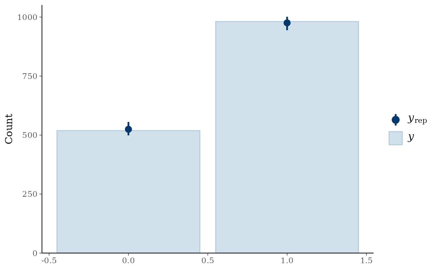
# Whether replicate outcomes look like the observed ones
if (rlang::is_installed("bayesplot")) {
  bayesplot::pp_check(fit, type = "bars")
}


# The scalar parameters and a spread of the predictor, as a draws array
if (rlang::is_installed("posterior")) {
  posterior::summarise_draws(posterior::as_draws(fit))
}
#> # A tibble: 12 × 10
#>    variable         mean   median     sd    mad       q5      q95  rhat ess_bulk
#>    <chr>           <dbl>    <dbl>  <dbl>  <dbl>    <dbl>    <dbl> <dbl>    <dbl>
#>  1 loglik       -8.37e+2 -8.36e+2 5.18   5.93   -845.    -828.    1.29      6.14
#>  2 sigma_mu.eta  4.67e-1  4.72e-1 0.0946 0.0901    0.343    0.659 1.13     13.7 
#>  3 eta[119]     -1.33e+0 -1.35e+0 0.286  0.231    -1.80    -0.844 1.04     51.1 
#>  4 eta[24]      -3.87e-1 -3.51e-1 0.434  0.469    -1.13     0.207 1.54      4.34
#>  5 eta[648]     -9.89e-4  1.71e-2 0.352  0.389    -0.591    0.488 1.16     14.1 
#>  6 eta[1432]     2.74e-1  2.58e-1 0.264  0.266    -0.195    0.686 1.09     18.1 
#>  7 eta[975]      5.48e-1  5.83e-1 0.339  0.252    -0.156    1.04  1.24      7.41
#>  8 eta[1083]     8.23e-1  8.27e-1 0.345  0.313     0.302    1.36  0.995    36.4 
#>  9 eta[144]      1.28e+0  1.29e+0 0.285  0.329     0.848    1.73  1.21      7.97
#> 10 eta[347]      1.65e+0  1.65e+0 0.355  0.392     1.14     2.19  1.40      5.30
#> 11 eta[513]      2.00e+0  2.02e+0 0.471  0.453     1.16     2.77  1.46      4.66
#> 12 eta[1135]     2.99e+0  2.97e+0 0.422  0.467     2.38     3.71  1.39      5.18
#> # ℹ 1 more variable: ess_tail <dbl>