Estimate the average marginal effect function (AMEF)

amef() computes the average marginal effect function (AMEF), the derivative of the average dose-response function (ADRF). This computed from an adrf_curve object or from a fitting outcome model directly.

Usage

amef(x, eps = 1e-05)

Arguments

x

an adrf_curve object; the output of a call to adrf().

eps

numeric; the step size to use when calculating numerical derivatives. Default is 1e-5 (.00001). See Details.

Value

An object of class amef_curve, which inherits from effect_curve.

Details

The AMEF is calculated numerically using the central finite derivative formula:

$$\frac{df(x)}{dx} \approx \frac{f(x + e) - f(x - e)}{2e}$$

The values of the ADRF at the evaluation points are computed using a local polynomial regression as described at effect_curve. At the boundaries of the ADRF, one-sided derivatives are used.

See also

• adrf() for computing the ADRF

• plot.effect_curve() for plotting the AMEF

• summary.effect_curve() for testing hypotheses about the AMEF

• effect_curve for computing point estimates along the AMEF

• curve_projection() for projecting a simpler model onto the AMEF

• reference_curve() for computing the difference between each point on the AMEF and a specific reference point

• curve_contrast() for contrasting AMEFs computed within subgroups

• marginaleffects::avg_slopes() for computing average adjusted slopes for fitted models (similar to the AMEF)

Examples

data("nhanes3lead")

fit <- lm(Math ~ poly(logBLL, 5) *
            Male * (Age + Race + PIR +
                      Enough_Food),
          data = nhanes3lead)

# ADRF of logBLL on Math
adrf1 <- adrf(fit, treat = "logBLL")

# AMEF of logBLL on Math
amef1 <- amef(adrf1)

amef1
#> An <effect_curve> object
#> 
#>  - curve type: AMEF
#>  - response: Math
#>  - treatment: logBLL
#>    + range: -0.3567 to 2.4248
#>  - inference: unconditional
#> 

# Plot the AMEF
plot(amef1)


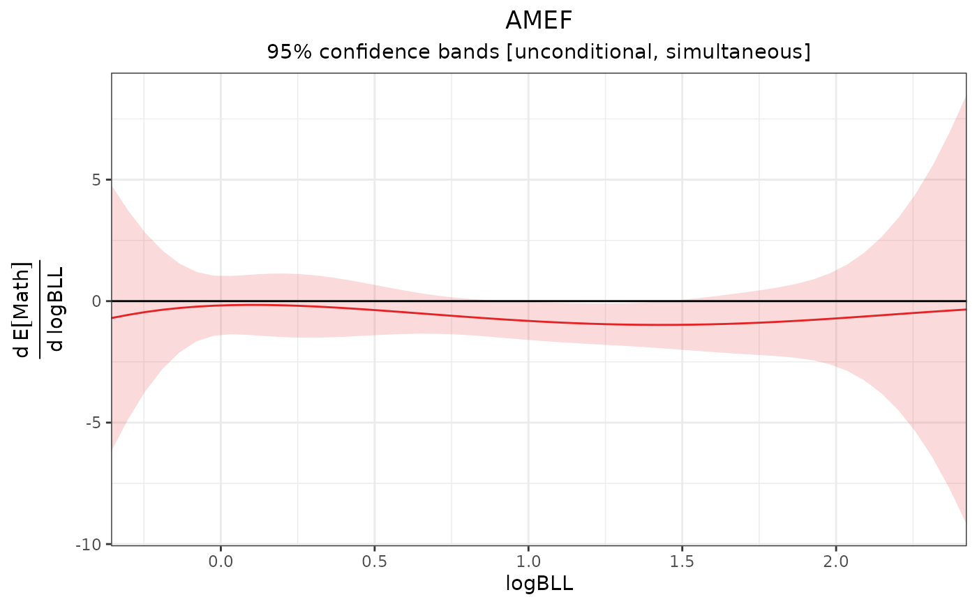# AMEF estimates at given points
amef1(logBLL = c(0, 1, 2)) |>
  summary()
#>                       AMEF Estimates
#> ───────────────────────────────────────────────────────────
#>  logBLL Estimate Std. Error       t P-value  CI Low CI High
#>       0  -0.1768     0.4286 -0.4125  0.9549 -1.1854  0.8319
#>       1  -0.8144     0.2780 -2.9297  0.0097 -1.4687 -0.1601
#>       2  -0.7111     0.7004 -1.0152  0.6160 -2.3597  0.9374
#> ───────────────────────────────────────────────────────────
#> Inference: unconditional, simultaneous
#> Confidence level: 95% (t* = 2.354, df = 2437)
#> Null value: 0