Summarize, print, and plot information about estimated weights

These functions summarize the weights resulting from a call to optweight() or optweight.svy(). summary() produces summary statistics on the distribution of weights, including their range and variability, and the effective sample size of the weighted sample (computing using the formula in McCaffrey, Rudgeway, & Morral, 2004). plot() creates a histogram of the weights.

Usage

# S3 method for class 'optweight'
summary(object, top = 5, ignore.s.weights = FALSE, weight.range = TRUE, ...)

# S3 method for class 'optweightMV'
summary(object, top = 5, ignore.s.weights = FALSE, weight.range = TRUE, ...)

# S3 method for class 'optweight.svy'
summary(object, top = 5, ignore.s.weights = FALSE, weight.range = TRUE, ...)

# S3 method for class 'summary.optweight'
plot(x, ...)

Arguments

object: An optweight, optweightMV, or optweight.svy object; the output of a call to optweight() or optweight.svy().
top: How many of the largest and smallest weights to display. Default is 5.
ignore.s.weights: Whether or not to ignore sampling weights when computing the weight summary. If FALSE, the default, the estimated weights will be multiplied by the sampling weights (if any) before values are computed.
weight.range: logical; whether display statistics about the range of weights and the highest and lowest weights for each group. Default is TRUE.
...: Additional arguments. For plot(), additional arguments passed to graphics::hist() to determine the number of bins, though ggplot2::geom_histogram() from ggplot2 is actually used to create the plot.
x: A summary.optweight, summary.optweightMV, or summary.optweight.svy object; the output of a call to summary.optweight(), summary.optweightMV(), or ()summary.optweight.svy.

Value

For point treatments (i.e., optweight objects), summary() returns a summary.optweight object with the following elements:

weight.range: The range (minimum and maximum) weight for each treatment group.
weight.top: The units with the greatest weights in each treatment group; how many are included is determined by top.
l2: The square root of the L2 norm of the estimated weights from the base weights, weighted by the sampling weights (if any): \(\sqrt{\frac{1}{n}\sum_i {s_i(w_i - b_i)^2}}\)
l1: The L1 norm of the estimated weights from the base weights, weighted by the sampling weights (if any): \(\frac{1}{n}\sum_i {s_i \vert w_i - b_i \vert}\)
linf: The L\(\infty\) norm (maximum absolute deviation) of the estimated weights from the base weights: \(\max_i {\vert w_i - b_i \vert}\)
rel.ent: The relative entropy between the estimated weights and the base weights (entropy norm), weighted by the sampling weights (if any): \(\frac{1}{n}\sum_i {s_i w_i \log\left(\frac{w_i}{b_i}\right)}\). Only computed if all weights are positive.
num.zeros: The number of units with a weight equal to 0.
effective.sample.size: The effective sample size for each treatment group before and after weighting.

For multivariate treatments (i.e., optweightMV objects), a list of the above elements for each treatment.

For optweight.svy objects, a list of the above elements but with no treatment group divisions.

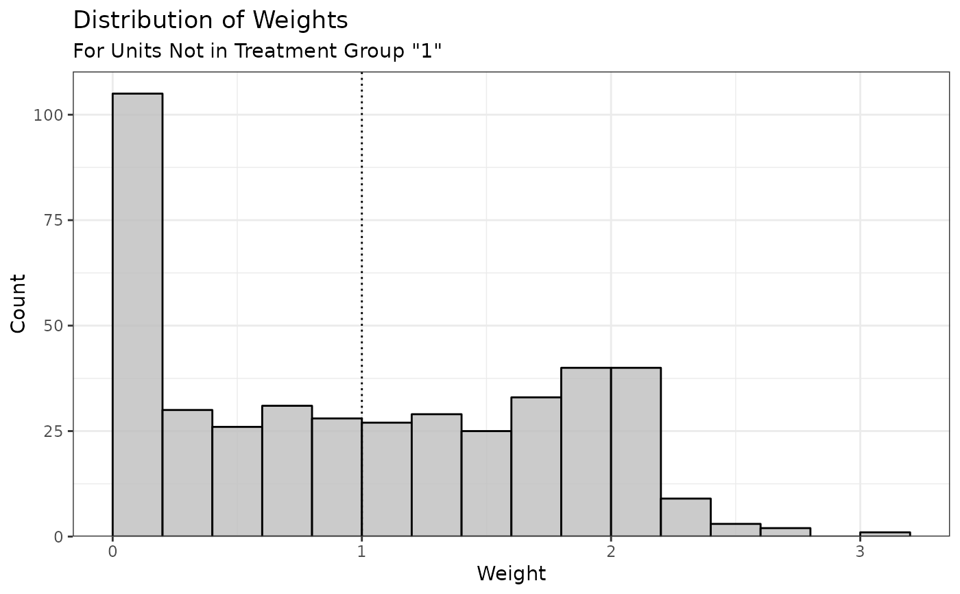
plot() returns a ggplot object with a histogram displaying the distribution of the estimated weights. If the estimand is the ATT or ATC, only the weights for the non-focal group(s) will be displayed (since the weights for the focal group are all 1). A dotted line is displayed at the mean of the weights (the mean of the base weights, or 1 if not supplied).

References

McCaffrey, D. F., Ridgeway, G., & Morral, A. R. (2004). Propensity Score Estimation With Boosted Regression for Evaluating Causal Effects in Observational Studies. Psychological Methods, 9(4), 403–425. doi:10.1037/1082-989X.9.4.403

Examples

library("cobalt")
data("lalonde", package = "cobalt")

#Balancing covariates between treatment groups (binary)
(ow1 <- optweight(treat ~ age + educ + married +
                    nodegree + re74, data = lalonde,
                  tols = .001,
                  estimand = "ATT"))
#> An optweight object
#>  - number of obs.: 614
#>  - norm minimized: "l2"
#>  - sampling weights: present
#>  - base weights: present
#>  - treatment: 2-category
#>  - estimand: ATT (focal: 1)
#>  - covariates: age, educ, married, nodegree, re74

(s <- summary(ow1))
#> Summary of weights:
#> 
#> - Weight ranges:
#>         Min                                  Max
#> treated   1           ||                  1.    
#> control   0 |---------------------------| 3.0186
#> 
#> - Units with 5 greatest weights by group:
#>                                            
#>               1      2      3      4      5
#>  treated      1      1      1      1      1
#>             404    226    224    111     84
#>  control 2.5106 2.5273 2.6258 2.7208 3.0186
#> 
#>            L2    L1    L∞ Rel Ent # Zeros
#> treated 0.    0.    0.       0.         0
#> control 0.783 0.694 2.019    0.39       0
#> 
#> - Effective Sample Sizes:
#>            Control Treated
#> Unweighted  429.       185
#> Weighted    265.88     185
#> 

plot(s, breaks = 12)