Plots the dual variables resulting from optweight(), optweightMV(), or optweight.svy() in a way similar to figure 2 of Zubizarreta (2015), which explains how to interpret these values.
Arguments
- x
an
optweight,optweightMV, oroptweight.svyobject; the output of a call tooptweight(),optweightMV(), oroptweight.svy().- type
the type of plot to display; allowable options include
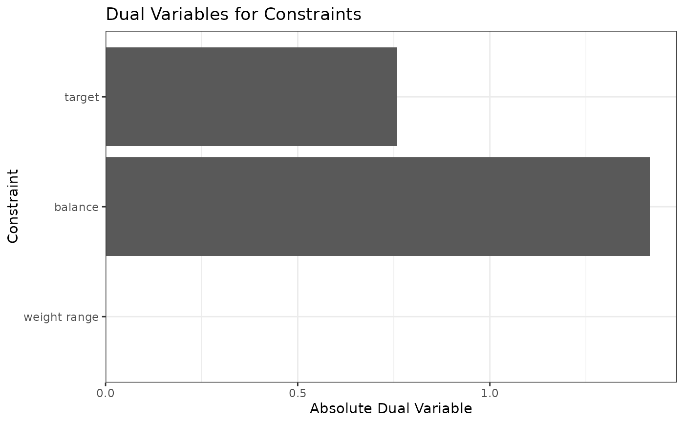
"variables"(the default), which produces a row for each covariate, and"constraints", which produces a row for each type of constraint (computed as the sum of the absolute dual variables for each constraint type).- ...
ignored.
- which.treat
for
optweightMVobjects, an integer corresponding to which treatment to display. Only one may be displayed at a time.
Details
Dual variables represent the cost of changing the constraint on the objective function minimized to estimate the weights. For covariates with large values of the dual variable, tightening the constraint will increase the variability of the weights, and relaxing the constraint will decrease the variability of the weights, both to a greater extent than would doing the same for covariate with small values of the dual variable. See optweight() and vignette("optweight") for more information on interpreting dual variables.
References
Zubizarreta, J. R. (2015). Stable Weights that Balance Covariates for Estimation With Incomplete Outcome Data. Journal of the American Statistical Association, 110(511), 910–922. doi:10.1080/01621459.2015.1023805
See also
optweight(), optweightMV(), or optweight.svy() to estimate the weights and the dual variables.
plot.summary.optweight() for plots of the distribution of weights.
Examples
library("cobalt")
data("lalonde", package = "cobalt")
tols <- process_tols(treat ~ age + educ + married +
nodegree + re74, data = lalonde,
tols = .1)
#Balancing covariates between treatment groups (binary)
ow1 <- optweight(treat ~ age + educ + married +
nodegree + re74, data = lalonde,
tols = tols,
estimand = "ATT")
# Note the L2 divergence and effective sample
# size (ESS)
summary(ow1, weight.range = FALSE)
#> Summary of weights
#>
#> - Weight statistics:
#>
#> L2 L1 L∞ Rel Ent # Zeros
#> treated 0. 0. 0 0. 0
#> control 0.532 0.462 1 0.181 0
#>
#> - Effective Sample Sizes:
#>
#> Control Treated
#> Unweighted 429. 185
#> Weighted 334.41 185
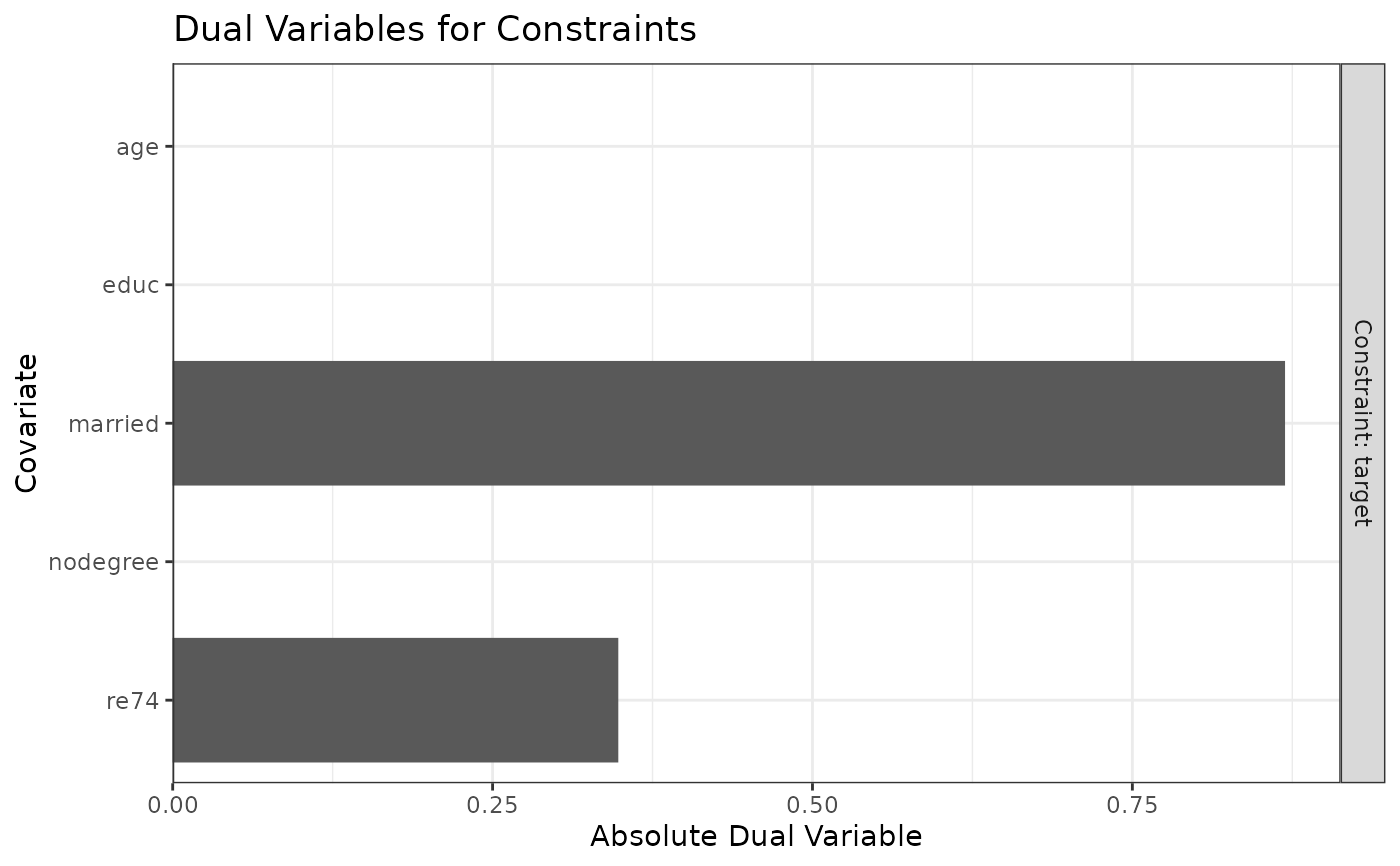
# age has a low value, married is high
plot(ow1)
 tols["age"] <- 0
ow2 <- optweight(treat ~ age + educ + married +
nodegree + re74, data = lalonde,
tols = tols,
estimand = "ATT")
# Notice that tightening the constraint on age has
# a negligible effect on the variability of the
# weights and ESS
summary(ow2, weight.range = FALSE)
#> Summary of weights
#>
#> - Weight statistics:
#>
#> L2 L1 L∞ Rel Ent # Zeros
#> treated 0. 0. 0 0. 0
#> control 0.534 0.465 1 0.183 0
#>
#> - Effective Sample Sizes:
#>
#> Control Treated
#> Unweighted 429. 185
#> Weighted 333.86 185
tols["age"] <- .1
tols["married"] <- 0
ow3 <- optweight(treat ~ age + educ + married +
nodegree + re74, data = lalonde,
tols = tols,
estimand = "ATT")
# In contrast, tightening the constraint on married
# has a large effect on the variability of the
# weights, shrinking the ESS
summary(ow3, weight.range = FALSE)
#> Summary of weights
#>
#> - Weight statistics:
#>
#> L2 L1 L∞ Rel Ent # Zeros
#> treated 0. 0. 0 0. 0
#> control 0.676 0.647 1 0.277 0
#>
#> - Effective Sample Sizes:
#>
#> Control Treated
#> Unweighted 429. 185
#> Weighted 294.35 185
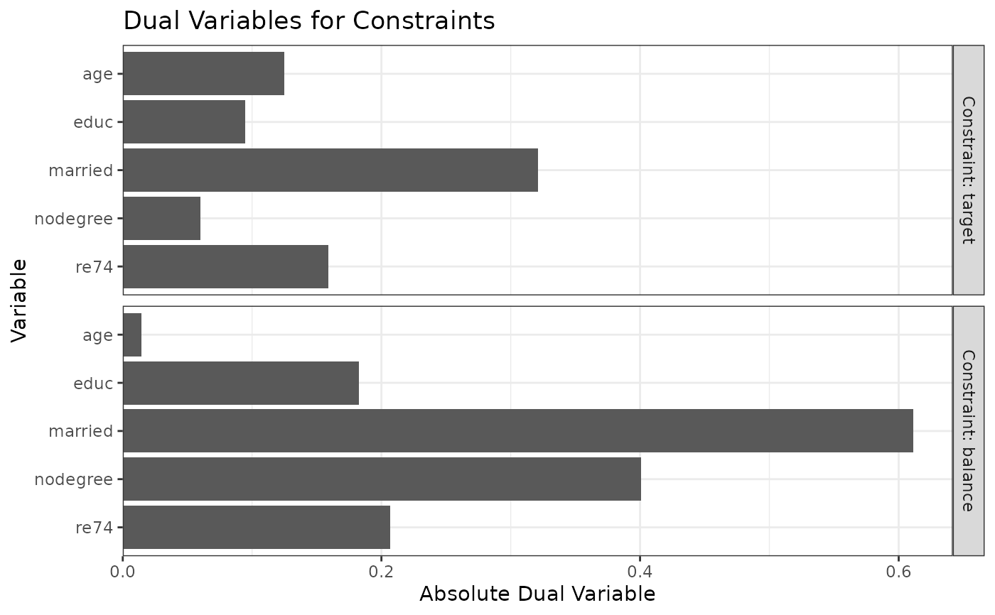
# More duals are displayed when targeting other
# estimands:
ow4 <- optweight(treat ~ age + educ + married +
nodegree + re74, data = lalonde,
estimand = "ATE")
plot(ow4)
tols["age"] <- 0
ow2 <- optweight(treat ~ age + educ + married +
nodegree + re74, data = lalonde,
tols = tols,
estimand = "ATT")
# Notice that tightening the constraint on age has
# a negligible effect on the variability of the
# weights and ESS
summary(ow2, weight.range = FALSE)
#> Summary of weights
#>
#> - Weight statistics:
#>
#> L2 L1 L∞ Rel Ent # Zeros
#> treated 0. 0. 0 0. 0
#> control 0.534 0.465 1 0.183 0
#>
#> - Effective Sample Sizes:
#>
#> Control Treated
#> Unweighted 429. 185
#> Weighted 333.86 185
tols["age"] <- .1
tols["married"] <- 0
ow3 <- optweight(treat ~ age + educ + married +
nodegree + re74, data = lalonde,
tols = tols,
estimand = "ATT")
# In contrast, tightening the constraint on married
# has a large effect on the variability of the
# weights, shrinking the ESS
summary(ow3, weight.range = FALSE)
#> Summary of weights
#>
#> - Weight statistics:
#>
#> L2 L1 L∞ Rel Ent # Zeros
#> treated 0. 0. 0 0. 0
#> control 0.676 0.647 1 0.277 0
#>
#> - Effective Sample Sizes:
#>
#> Control Treated
#> Unweighted 429. 185
#> Weighted 294.35 185
# More duals are displayed when targeting other
# estimands:
ow4 <- optweight(treat ~ age + educ + married +
nodegree + re74, data = lalonde,
estimand = "ATE")
plot(ow4)
 # Display duals by constraint type
plot(ow4, type = "constraints")
# Display duals by constraint type
plot(ow4, type = "constraints")