This page explains the details of estimating weights from
generalized boosted model-based propensity scores by setting method = "gbm"
in the call to weightit() or weightitMSM(). This method can be used with
binary, multi-category, and continuous treatments.
In general, this method relies on estimating propensity scores using generalized boosted modeling and then converting those propensity scores into weights using a formula that depends on the desired estimand. The algorithm involves using a balance-based or prediction-based criterion to optimize in choosing the value of tuning parameters (the number of trees and possibly others). The method relies on the gbm package.
This method mimics the functionality of functions in the twang package, but has improved performance and more flexible options. See Details section for more details.
Binary Treatments
For binary treatments, this method estimates the propensity scores using
gbm::gbm.fit()
and then selects the optimal tuning parameter values
using the method specified in the criterion argument. The following
estimands are allowed: ATE, ATT, ATC, ATO, and ATM. The weights are computed
from the estimated propensity scores using get_w_from_ps(), which
implements the standard formulas. Weights can also be computed using marginal
mean weighting through stratification for the ATE, ATT, and ATC. See
get_w_from_ps() for details.
Multi-Category Treatments
For binary treatments, this method estimates the propensity scores using
gbm::gbm.fit()
and then selects the optimal tuning parameter values
using the method specified in the criterion argument. The following
estimands are allowed: ATE, ATT, ATC, ATO, and ATM. The weights are computed
from the estimated propensity scores using get_w_from_ps(), which
implements the standard formulas. Weights can also be computed using marginal
mean weighting through stratification for the ATE, ATT, and ATC. See
get_w_from_ps() for details.
Continuous Treatments
For continuous treatments, this method estimates the generalized propensity
score using gbm::gbm.fit()
and then selects the optimal tuning
parameter values using the method specified in the criterion argument.
Longitudinal Treatments
For longitudinal treatments, the weights are the product of the weights estimated at each time point.
Missing Data
In the presence of missing data, the following value(s) for missing are allowed:
"ind"(default)Missing variables are automatically handled by the boosting model. When using a
criteriontargeting covariate balance, for each variable with missingness, a new missingness indicator variable is created which takes the value 1 if the original covariate isNAand 0 otherwise. The missingness indicators are included as covariate to balance. The missing values in the covariates are then replaced with the covariate medians. Balance assessment then proceeds with this new set of covariates. The covariates output in the resultingweightitobject will be the original covariates with theNAs.
Details
Generalized boosted modeling (GBM, also known as gradient boosting machines) is a machine learning method that generates predicted values from a flexible regression of the treatment on the covariates, which are treated as propensity scores and used to compute weights. It does this by building a series of regression trees, each fit to the residuals of the last, minimizing a loss function that depends on the distribution chosen. The optimal number of trees is a tuning parameter that must be chosen; McCaffrey et al. (2004) were innovative in using covariate balance to select this value rather than traditional machine learning performance metrics such as cross-validation accuracy. GBM is particularly effective for fitting nonlinear treatment models characterized by curves and interactions, but performs worse for simpler treatment models. It is unclear which balance measure should be used to select the number of trees, though research has indicated that balance measures tend to perform better than cross-validation accuracy for estimating effective propensity score weights.
WeightIt offers almost identical functionality to twang, the first package to implement this method. Compared to the current version of twang, WeightIt offers more options for the measure of balance used to select the number of trees, improved performance, tuning of hyperparameters, more estimands, and support for continuous treatments. WeightIt computes weights for multi-category treatments differently from how twang does; rather than fitting a separate binary GBM for each pair of treatments, WeightIt fits a single multi-class GBM model and uses balance measures appropriate for multi-category treatments.
plot() can be used on the output of weightit() with method = "gbm" to
display the results of the tuning process; see Examples and plot.weightit()
for more details.
Note
The criterion argument used to be called stop.method, which is its
name in twang. stop.method still works for backward compatibility.
Additionally, the criteria formerly named as "es.mean", "es.max", and
"es.rms" have been renamed to "smd.mean", "smd.max", and "smd.rms".
The former are used in twang and will still work with weightit() for
backward compatibility.
Estimated propensity scores are trimmed to \(10^{-8}\) and \(1 - 10^{-8}\) to ensure balance statistics can be computed.
An additional missing argument, "surr", used to be allowed; it is now set to "ind" with a warning.
Additional Arguments
The following additional arguments can be specified:
criterionA string describing the balance criterion used to select the best weights. See
cobalt::bal.compute()for allowable options for each treatment type. In addition, to optimize the cross-validation error instead of balance,criterioncan be set as"cv{#}", where{#}is replaced by a number representing the number of cross-validation folds used (e.g.,"cv5"for 5-fold cross-validation). For binary and multi-category treatments, the default is"smd.mean", which minimizes the average absolute standard mean difference among the covariates between treatment groups. For continuous treatments, the default is"p.mean", which minimizes the average absolute Pearson correlation between the treatment and covariates.trim.atA number supplied to
atintrim()which trims the weights from all the trees before choosing the best tree. This can be valuable when some weights are extreme, which occurs especially with continuous treatments. The default is 0 (i.e., no trimming).subclassinteger; the number of subclasses to use for computing weights using marginal mean weighting through stratification (MMWS). IfNULL, standard inverse probability weights (and their extensions) will be computed; if a number greater than 1, subclasses will be formed and weights will be computed based on subclass membership. Only allowed for binary and multi-category treatments. Seeget_w_from_ps()for details and references.distributionA string with the distribution used in the loss function of the boosted model. This is supplied to the
distributionargument ingbm::gbm.fit(). For binary treatments,"bernoulli"and"adaboost"are available, with"bernoulli"the default. For multi-category treatments, only"multinomial"is allowed. For continuous treatments"gaussian","laplace", and"tdist"are available, with"gaussian"the default. This argument is tunable.n.treesThe maximum number of trees used. This is passed onto the
n.treesargument ingbm.fit(). The default is 10000 for binary and multi-category treatments and 20000 for continuous treatments.start.treeThe tree at which to start balance checking. If you know the best balance isn't in the first 100 trees, for example, you can set
start.tree = 101so that balance statistics are not computed on the first 100 trees. This can save some time since balance checking takes up the bulk of the run time for some balance-based stopping methods, and is especially useful when running the same model adding more and more trees. The default is 1, i.e., to start from the very first tree in assessing balance.interaction.depthThe depth of the trees. This is passed onto the
interaction.depthargument ingbm.fit(). Higher values indicate better ability to capture nonlinear and nonadditive relationships. The default is 3 for binary and multi-category treatments and 4 for continuous treatments. This argument is tunable.shrinkageThe shrinkage parameter applied to the trees. This is passed onto the
shrinkageargument ingbm.fit(). The default is .01 for binary and multi-category treatments and .0005 for continuous treatments. The lower this value is, the more trees one may have to include to reach the optimum. This argument is tunable.bag.fractionThe fraction of the units randomly selected to propose the next tree in the expansion. This is passed onto the
bag.fractionargument ingbm.fit(). The default is 1, but smaller values should be tried. For values less then 1, subsequent runs with the same parameters will yield different results due to random sampling; be sure to seed the seed usingset.seed()to ensure replicability of results.use.offsetlogical; whether to use the linear predictor resulting from a generalized linear model as an offset to the GBM model. IfTRUE, this fits a logistic regression model (for binary treatments) or a linear regression model (for continuous treatments) and supplies the linear predict to theoffsetargument ofgbm.fit(). This often improves performance generally but especially when the true propensity score model is well approximated by a GLM, and this yields uniformly superior performance overmethod = "glm"with respect tocriterion. Default isFALSEto omit the offset. Only allowed for binary and continuous treatments. This argument is tunable.
All other arguments take on the defaults of those in gbm::gbm.fit()
,
and some are not used at all. For binary and multi-category treatments with
a with cross-validation used as the criterion, class.stratify.cv is set
to TRUE by default.
The w argument in gbm.fit() is ignored because sampling weights are
passed using s.weights.
For continuous treatments only, the following arguments may be supplied:
densityA function corresponding to the conditional density of the treatment. The standardized residuals of the treatment model will be fed through this function to produce the numerator and denominator of the generalized propensity score weights. This can also be supplied as a string containing the name of the function to be called. If the string contains underscores, the call will be split by the underscores and the latter splits will be supplied as arguments to the second argument and beyond. For example, if
density = "dt_2"is specified, the density used will be that of a t-distribution with 2 degrees of freedom. Using a t-distribution can be useful when extreme outcome values are observed (Naimi et al., 2014).Can also be
"kernel"to use kernel density estimation, which callsdensity()to estimate the numerator and denominator densities for the weights. (This used to be requested by settinguse.kernel = TRUE, which is now deprecated.)If unspecified, a density corresponding to the argument passed to
distribution. If"gaussian"(the default),dnorm()is used. If"tdist", a t-distribution with 4 degrees of freedom is used. If"laplace", a laplace distribution is used.bw,adjust,kernel,nIf
density = "kernel", the arguments todensity(). The defaults are the same as those indensity()except thatnis 10 times the number of units in the sample.plotIf
density = "kernel", whether to plot the estimated densities.
For tunable arguments, multiple entries may be supplied, and weightit()
will choose the best value by optimizing the criterion specified in
criterion. See below for additional outputs that are included when
arguments are supplied to be tuned. See Examples for an example of tuning.
The same seed is used for every run to ensure any variation in performance
across tuning parameters is due to the specification and not to using a
random seed. This only matters when bag.fraction differs from 1 (its
default) or cross-validation is used as the criterion; otherwise, there are
no random components in the model.
Additional Outputs
infoA list with the following entries:
best.treeThe number of trees at the optimum. If this is close to
n.trees,weightit()should be rerun with a larger value forn.trees, andstart.treecan be set to just belowbest.tree. When other parameters are tuned, this is the best tree value in the best combination of tuned parameters. See example.tree.valA data frame with two columns: the first is the number of trees and the second is the value of the criterion corresponding to that tree. When other parameters are tuned, these are the number of trees and the criterion values in the best combination of tuned parameters. See example.
If any arguments are to be tuned (i.e., they have been supplied more than one value), the following two additional components are included in
info:tuneA data frame with a column for each argument being tuned, the best value of the balance criterion for the given combination of parameters, and the number of trees at which the best value was reached.
best.tuneA one-row data frame containing the values of the arguments being tuned that were ultimately selected to estimate the returned weights.
objWhen
include.obj = TRUE, thegbmfit used to generate the predicted values.
References
Binary treatments
McCaffrey, D. F., Ridgeway, G., & Morral, A. R. (2004). Propensity Score Estimation With Boosted Regression for Evaluating Causal Effects in Observational Studies. Psychological Methods, 9(4), 403–425. doi:10.1037/1082-989X.9.4.403
Multi-Category Treatments
McCaffrey, D. F., Griffin, B. A., Almirall, D., Slaughter, M. E., Ramchand, R., & Burgette, L. F. (2013). A Tutorial on Propensity Score Estimation for Multiple Treatments Using Generalized Boosted Models. Statistics in Medicine, 32(19), 3388–3414. doi:10.1002/sim.5753
Continuous treatments
Zhu, Y., Coffman, D. L., & Ghosh, D. (2015). A Boosting Algorithm for Estimating Generalized Propensity Scores with Continuous Treatments. Journal of Causal Inference, 3(1). doi:10.1515/jci-2014-0022
See also
gbm::gbm.fit()
for the fitting function.
Examples
data("lalonde", package = "cobalt")
#Balancing covariates between treatment groups (binary)
(W1 <- weightit(treat ~ age + educ + married +
nodegree + re74, data = lalonde,
method = "gbm", estimand = "ATE",
criterion = "smd.max",
use.offset = TRUE))
#> A weightit object
#> - method: "gbm" (propensity score weighting with GBM)
#> - number of obs.: 614
#> - sampling weights: none
#> - treatment: 2-category
#> - estimand: ATE
#> - covariates: age, educ, married, nodegree, re74
summary(W1)
#> Summary of weights
#>
#> - Weight ranges:
#>
#> Min Max
#> treated 1.133 |---------------------------| 22.939
#> control 1.007 |------| 6.886
#>
#> - Units with the 5 most extreme weights by group:
#>
#> 181 177 183 184 182
#> treated 10.484 11.097 15.942 18.361 22.939
#> 409 592 569 374 608
#> control 3.913 3.978 4.087 4.151 6.886
#>
#> - Weight statistics:
#>
#> Coef of Var MAD Entropy # Zeros
#> treated 1.049 0.558 0.306 0
#> control 0.381 0.218 0.051 0
#>
#> - Effective Sample Sizes:
#>
#> Control Treated
#> Unweighted 429. 185.
#> Weighted 374.69 88.35
cobalt::bal.tab(W1)
#> Balance Measures
#> Type Diff.Adj
#> prop.score Distance 0.6920
#> age Contin. -0.1894
#> educ Contin. 0.0767
#> married Binary -0.0734
#> nodegree Binary 0.0249
#> re74 Contin. 0.1111
#>
#> Effective sample sizes
#> Control Treated
#> Unadjusted 429. 185.
#> Adjusted 374.69 88.35
# View information about the fitting process
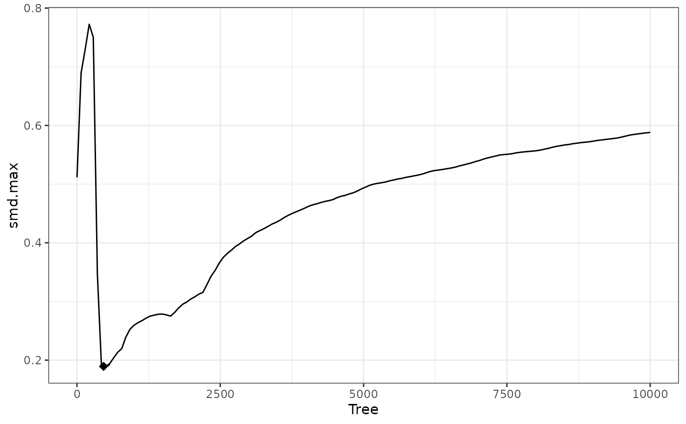
W1$info$best.tree #best tree
#> 1
#> 464
plot(W1) #plot of criterion value against number of trees
 #Balancing covariates with respect to race (multi-category)
(W2 <- weightit(race ~ age + educ + married +
nodegree + re74, data = lalonde,
method = "gbm", estimand = "ATT",
focal = "hispan", criterion = "ks.mean"))
#> A weightit object
#> - method: "gbm" (propensity score weighting with GBM)
#> - number of obs.: 614
#> - sampling weights: none
#> - treatment: 3-category (black, hispan, white)
#> - estimand: ATT (focal: hispan)
#> - covariates: age, educ, married, nodegree, re74
summary(W2)
#> Summary of weights
#>
#> - Weight ranges:
#>
#> Min Max
#> black 0.067 |------------------------| 1.059
#> hispan 1. || 1.
#> white 0.037 |---------------------------| 1.152
#>
#> - Units with the 5 most extreme weights by group:
#>
#> 183 162 191 485 190
#> black 0.908 0.954 0.954 1.043 1.059
#> 100 87 44 28 2
#> hispan 1 1 1 1 1
#> 68 227 380 434 523
#> white 0.688 0.721 0.813 0.834 1.152
#>
#> - Weight statistics:
#>
#> Coef of Var MAD Entropy # Zeros
#> black 0.719 0.523 0.211 0
#> hispan 0. 0. 0. 0
#> white 0.641 0.483 0.18 0
#>
#> - Effective Sample Sizes:
#>
#> black hispan white
#> Unweighted 243. 72 299.
#> Weighted 160.38 72 212.12
cobalt::bal.tab(W2, stats = c("m", "ks"))
#> Balance summary across all treatment pairs
#> Type Max.Diff.Adj Max.KS.Adj
#> age Contin. 0.0823 0.0887
#> educ Contin. 0.2987 0.1272
#> married Binary 0.1170 0.1170
#> nodegree Binary 0.0658 0.0658
#> re74 Contin. 0.0308 0.0934
#>
#> Effective sample sizes
#> black white hispan
#> Unadjusted 243. 299. 72
#> Adjusted 160.38 212.12 72
#Balancing covariates with respect to re75 (continuous)
(W3 <- weightit(re75 ~ age + educ + married +
nodegree + re74, data = lalonde,
method = "gbm", density = "kernel",
criterion = "p.rms", trim.at = .97))
#> A weightit object
#> - method: "gbm" (propensity score weighting with GBM)
#> - number of obs.: 614
#> - sampling weights: none
#> - treatment: continuous
#> - covariates: age, educ, married, nodegree, re74
summary(W3)
#> Summary of weights
#>
#> - Weight ranges:
#>
#> Min Max
#> all 0.07 |---------------------------| 11.818
#>
#> - Units with the 5 most extreme weights:
#>
#> 407 395 375 354 308
#> all 11.818 11.818 11.818 11.818 11.818
#>
#> - Weight statistics:
#>
#> Coef of Var MAD Entropy # Zeros
#> all 1.244 0.839 0.524 0
#>
#> - Effective Sample Sizes:
#>
#> Total
#> Unweighted 614.
#> Weighted 241.25
cobalt::bal.tab(W3)
#> Balance Measures
#> Type Corr.Adj
#> age Contin. 0.0031
#> educ Contin. 0.0158
#> married Binary 0.0410
#> nodegree Binary -0.0242
#> re74 Contin. 0.0927
#>
#> Effective sample sizes
#> Total
#> Unadjusted 614.
#> Adjusted 241.25
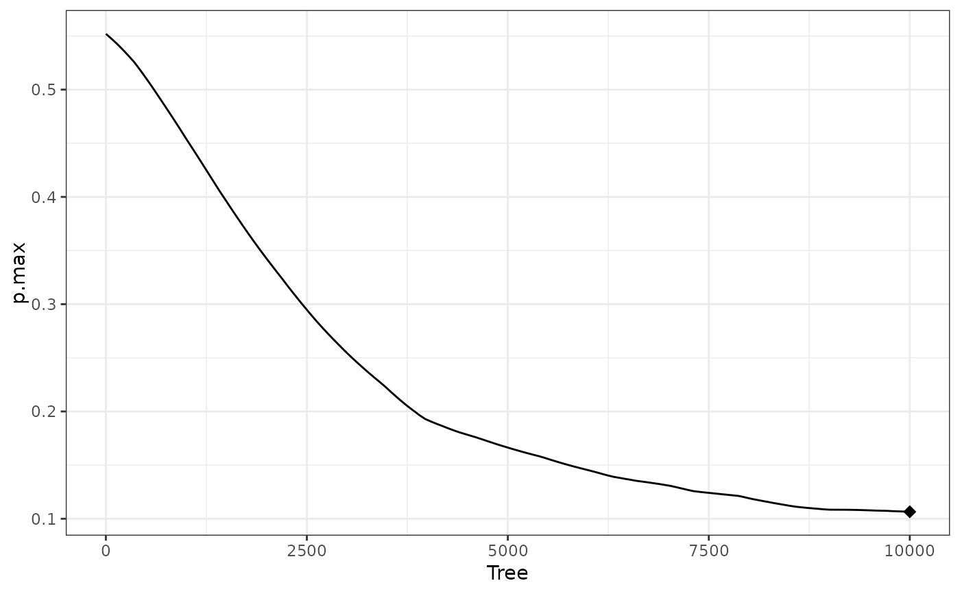
#Using a t(3) density and illustrating the search for
#more trees.
W4a <- weightit(re75 ~ age + educ + married +
nodegree + re74, data = lalonde,
method = "gbm", density = "dt_3",
criterion = "p.max",
n.trees = 10000)
W4a$info$best.tree #10000; optimum hasn't been found
#> 1
#> 10000
plot(W4a) #decreasing at right edge
#Balancing covariates with respect to race (multi-category)
(W2 <- weightit(race ~ age + educ + married +
nodegree + re74, data = lalonde,
method = "gbm", estimand = "ATT",
focal = "hispan", criterion = "ks.mean"))
#> A weightit object
#> - method: "gbm" (propensity score weighting with GBM)
#> - number of obs.: 614
#> - sampling weights: none
#> - treatment: 3-category (black, hispan, white)
#> - estimand: ATT (focal: hispan)
#> - covariates: age, educ, married, nodegree, re74
summary(W2)
#> Summary of weights
#>
#> - Weight ranges:
#>
#> Min Max
#> black 0.067 |------------------------| 1.059
#> hispan 1. || 1.
#> white 0.037 |---------------------------| 1.152
#>
#> - Units with the 5 most extreme weights by group:
#>
#> 183 162 191 485 190
#> black 0.908 0.954 0.954 1.043 1.059
#> 100 87 44 28 2
#> hispan 1 1 1 1 1
#> 68 227 380 434 523
#> white 0.688 0.721 0.813 0.834 1.152
#>
#> - Weight statistics:
#>
#> Coef of Var MAD Entropy # Zeros
#> black 0.719 0.523 0.211 0
#> hispan 0. 0. 0. 0
#> white 0.641 0.483 0.18 0
#>
#> - Effective Sample Sizes:
#>
#> black hispan white
#> Unweighted 243. 72 299.
#> Weighted 160.38 72 212.12
cobalt::bal.tab(W2, stats = c("m", "ks"))
#> Balance summary across all treatment pairs
#> Type Max.Diff.Adj Max.KS.Adj
#> age Contin. 0.0823 0.0887
#> educ Contin. 0.2987 0.1272
#> married Binary 0.1170 0.1170
#> nodegree Binary 0.0658 0.0658
#> re74 Contin. 0.0308 0.0934
#>
#> Effective sample sizes
#> black white hispan
#> Unadjusted 243. 299. 72
#> Adjusted 160.38 212.12 72
#Balancing covariates with respect to re75 (continuous)
(W3 <- weightit(re75 ~ age + educ + married +
nodegree + re74, data = lalonde,
method = "gbm", density = "kernel",
criterion = "p.rms", trim.at = .97))
#> A weightit object
#> - method: "gbm" (propensity score weighting with GBM)
#> - number of obs.: 614
#> - sampling weights: none
#> - treatment: continuous
#> - covariates: age, educ, married, nodegree, re74
summary(W3)
#> Summary of weights
#>
#> - Weight ranges:
#>
#> Min Max
#> all 0.07 |---------------------------| 11.818
#>
#> - Units with the 5 most extreme weights:
#>
#> 407 395 375 354 308
#> all 11.818 11.818 11.818 11.818 11.818
#>
#> - Weight statistics:
#>
#> Coef of Var MAD Entropy # Zeros
#> all 1.244 0.839 0.524 0
#>
#> - Effective Sample Sizes:
#>
#> Total
#> Unweighted 614.
#> Weighted 241.25
cobalt::bal.tab(W3)
#> Balance Measures
#> Type Corr.Adj
#> age Contin. 0.0031
#> educ Contin. 0.0158
#> married Binary 0.0410
#> nodegree Binary -0.0242
#> re74 Contin. 0.0927
#>
#> Effective sample sizes
#> Total
#> Unadjusted 614.
#> Adjusted 241.25
#Using a t(3) density and illustrating the search for
#more trees.
W4a <- weightit(re75 ~ age + educ + married +
nodegree + re74, data = lalonde,
method = "gbm", density = "dt_3",
criterion = "p.max",
n.trees = 10000)
W4a$info$best.tree #10000; optimum hasn't been found
#> 1
#> 10000
plot(W4a) #decreasing at right edge
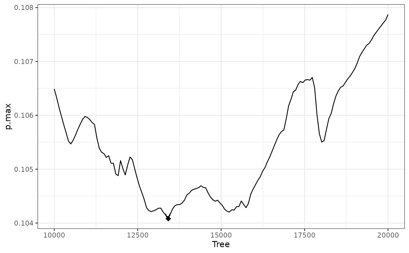
 W4b <- weightit(re75 ~ age + educ + married +
nodegree + re74, data = lalonde,
method = "gbm", density = "dt_3",
criterion = "p.max",
start.tree = 10000,
n.trees = 20000)
W4b$info$best.tree #13417; optimum has been found
#> 1
#> 13417
plot(W4b) #increasing at right edge
W4b <- weightit(re75 ~ age + educ + married +
nodegree + re74, data = lalonde,
method = "gbm", density = "dt_3",
criterion = "p.max",
start.tree = 10000,
n.trees = 20000)
W4b$info$best.tree #13417; optimum has been found
#> 1
#> 13417
plot(W4b) #increasing at right edge
 cobalt::bal.tab(W4b)
#> Balance Measures
#> Type Corr.Adj
#> age Contin. 0.0362
#> educ Contin. 0.0502
#> married Binary 0.0717
#> nodegree Binary -0.0665
#> re74 Contin. 0.1041
#>
#> Effective sample sizes
#> Total
#> Unadjusted 614.
#> Adjusted 251.08
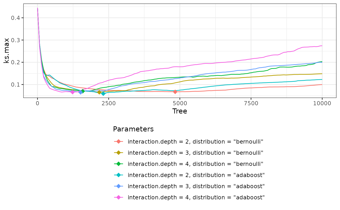
#Tuning hyperparameters
(W5 <- weightit(treat ~ age + educ + married +
nodegree + re74, data = lalonde,
method = "gbm", estimand = "ATT",
criterion = "ks.max",
interaction.depth = 2:4,
distribution = c("bernoulli", "adaboost")))
#> A weightit object
#> - method: "gbm" (propensity score weighting with GBM)
#> - number of obs.: 614
#> - sampling weights: none
#> - treatment: 2-category
#> - estimand: ATT (focal: 1)
#> - covariates: age, educ, married, nodegree, re74
W5$info$tune
#> interaction.depth shrinkage distribution use.offset best.ks.max best.tree
#> 1 2 0.01 bernoulli FALSE 0.06704768 4836
#> 2 3 0.01 bernoulli FALSE 0.06517037 2171
#> 3 4 0.01 bernoulli FALSE 0.06988698 1588
#> 4 2 0.01 adaboost FALSE 0.05894705 2311
#> 5 3 0.01 adaboost FALSE 0.06485408 1514
#> 6 4 0.01 adaboost FALSE 0.06591365 1232
W5$info$best.tune #Best values of tuned parameters
#> interaction.depth shrinkage distribution use.offset best.ks.max best.tree
#> 4 2 0.01 adaboost FALSE 0.05894705 2311
plot(W5) #plot criterion values against number of trees
cobalt::bal.tab(W4b)
#> Balance Measures
#> Type Corr.Adj
#> age Contin. 0.0362
#> educ Contin. 0.0502
#> married Binary 0.0717
#> nodegree Binary -0.0665
#> re74 Contin. 0.1041
#>
#> Effective sample sizes
#> Total
#> Unadjusted 614.
#> Adjusted 251.08
#Tuning hyperparameters
(W5 <- weightit(treat ~ age + educ + married +
nodegree + re74, data = lalonde,
method = "gbm", estimand = "ATT",
criterion = "ks.max",
interaction.depth = 2:4,
distribution = c("bernoulli", "adaboost")))
#> A weightit object
#> - method: "gbm" (propensity score weighting with GBM)
#> - number of obs.: 614
#> - sampling weights: none
#> - treatment: 2-category
#> - estimand: ATT (focal: 1)
#> - covariates: age, educ, married, nodegree, re74
W5$info$tune
#> interaction.depth shrinkage distribution use.offset best.ks.max best.tree
#> 1 2 0.01 bernoulli FALSE 0.06704768 4836
#> 2 3 0.01 bernoulli FALSE 0.06517037 2171
#> 3 4 0.01 bernoulli FALSE 0.06988698 1588
#> 4 2 0.01 adaboost FALSE 0.05894705 2311
#> 5 3 0.01 adaboost FALSE 0.06485408 1514
#> 6 4 0.01 adaboost FALSE 0.06591365 1232
W5$info$best.tune #Best values of tuned parameters
#> interaction.depth shrinkage distribution use.offset best.ks.max best.tree
#> 4 2 0.01 adaboost FALSE 0.05894705 2311
plot(W5) #plot criterion values against number of trees
 cobalt::bal.tab(W5, stats = c("m", "ks"))
#> Balance Measures
#> Type Diff.Adj KS.Adj
#> prop.score Distance 0.2909 0.1727
#> age Contin. 0.0596 0.0589
#> educ Contin. -0.0006 0.0547
#> married Binary -0.0135 0.0135
#> nodegree Binary 0.0547 0.0547
#> re74 Contin. 0.0683 0.0309
#>
#> Effective sample sizes
#> Control Treated
#> Unadjusted 429. 185
#> Adjusted 42.01 185
cobalt::bal.tab(W5, stats = c("m", "ks"))
#> Balance Measures
#> Type Diff.Adj KS.Adj
#> prop.score Distance 0.2909 0.1727
#> age Contin. 0.0596 0.0589
#> educ Contin. -0.0006 0.0547
#> married Binary -0.0135 0.0135
#> nodegree Binary 0.0547 0.0547
#> re74 Contin. 0.0683 0.0309
#>
#> Effective sample sizes
#> Control Treated
#> Unadjusted 429. 185
#> Adjusted 42.01 185