Fractional Weighted Bootstrap

fwb() implements the fractional (random) weighted bootstrap, also known as the Bayesian bootstrap. Rather than resampling units to include in bootstrap samples, weights are drawn to be applied to a weighted estimator.

Usage

fwb(
  data,
  statistic,
  R = 999,
  cluster = NULL,
  simple = FALSE,
  wtype = getOption("fwb_wtype", "exp"),
  verbose = TRUE,
  cl = NULL,
  ...
)

# S3 method for fwb
print(x, digits = getOption("digits"), index = 1L:ncol(x$t), ...)

Arguments

data: the dataset used to compute the statistic
statistic: a function, which, when applied to data, returns a vector containing the statistic(s) of interest. The function should take at least two arguments; the first argument should correspond to the dataset and the second argument should correspond to a vector of weights. Any further arguments can be passed to statistic through the ... argument.
R: the number of bootstrap replicates. Default is 999 but more is always better. For the percentile bootstrap confidence interval to be exact, it can be beneficial to use one less than a multiple of 100.
cluster: optional; a vector containing cluster membership. If supplied, will run the cluster bootstrap. See Details. Evaluated first in data and then in the global environment.
simple: logical; if TRUE, weights will be computed on-the-fly in each bootstrap replication rather than all at once. This can save memory at the cost of some speed.
wtype: string; the type of weights to use. Allowable options include "exp" (the default), "pois", "multinom", and "mammen". See Details. See set_fwb_wtype() to set a global default.
verbose: logical; whether to display a progress bar.
cl: a cluster object created by parallel::makeCluster(), or an integer to indicate the number of child-processes (integer values are ignored on Windows) for parallel evaluations. See pbapply::pblapply() for details. If NULL, no parallelization will take place.
...: other arguments passed to statistic.
x: an fwb object; the output of a call to fwb().
digits: the number of significant digits to print
index: the index or indices of the position of the quantity of interest in x$t0 if more than one was specified in fwb(). Default is to print all quantities.

Value

A fwb object, which also inherits from boot, with the following components:

t0: The observed value of statistic applied to data with uniform weights.
t: A matrix with R rows, each of which is a bootstrap replicate of the result of calling statistic.
R: The value of R as passed to fwb().
data: The data as passed to fwb().
seed: The value of .Random.seed just prior to generating the weights (after the first call to statistic with uniform weights).
statistic: The function statistic as passed to fwb().
call: The original call to fwb().
cluster: The vector passed to cluster, if any.
wtype: The type of weights used as determined by the wtype argument.

Details

fwb() implements the fractional weighted bootstrap and is meant to function as a drop-in for boot::boot(., stype = "f") (i.e., the usual bootstrap but with frequency weights representing the number of times each unit is drawn). In each bootstrap replication, when wtype = "exp" (the default), the weights are sampled from independent exponential distributions with rate parameter 1 and then normalized to have a mean of 1, equivalent to drawing the weights from a Dirichlet distribution. Other weights are allowed as determined by the wtype argument (see set_fwb_wtype() for details). The function supplied to statistic must incorporate the weights to compute a weighted statistic. For example, if the output is a regression coefficient, the weights supplied to the w argument of statistic should be supplied to the weights argument of lm(). These weights should be used any time frequency weights would be, since they are meant to function like frequency weights (which, in the case of the traditional bootstrap, would be integers). Unfortunately, there is no way for fwb() to know whether you are using the weights correctly, so care should be taken to ensure weights are correctly incorporated into the estimator.

When fitting binomial regression models (e.g., logistic) using glm(), it may be useful to change the family to a "quasi" variety (e.g., quasibinomial()) to avoid a spurious warning about "non-integer #successes".

The cluster bootstrap can be requested by supplying a vector of cluster membership to cluster. Rather than generating a weight for each unit, a weight is generated for each cluster and then applied to all units in that cluster.

Ideally, statistic should not involve a random element, or else it will not be straightforward to replicate the bootstrap results using the seed included in the output object. Setting a seed using set.seed() is always advised.

The print() method displays the value of the statistics, the bias (the difference between the statistic and the mean of its bootstrap distribution), and the standard error (the standard deviation of the bootstrap distribution).

Weight types

Different types of weights can be supplied to the wtype argument. A global default can be set using set_fwb_wtype(). The allowable weight types are described below.

"exp"

Draws weights from an exponential distribution with rate parameter 1 using rexp(). These weights are the usual "Bayesian bootstrap" weights described in Xu et al. (2020). They are equivalent to drawing weights from a uniform Dirichlet distribution, which is what gives these weights the interpretation of a Bayesian prior.

"multinom"

Draws integer weights using sample(), which samples unit indices with replacement and uses the tabulation of the indices as frequency weights. This is equivalent to drawing weights from a multinomial distribution. Using wtype = "multinom" is the same as using boot::boot(., stype = "f") instead of fwb() (i.e., the resulting estimates will be identical).

"poisson"

Draws integer weights from a Poisson distribution with 1 degree of freedom using rpois(). This is an alternative to the multinomial weights that yields similar estimates (especially as the sample size grows) but can be faster.

"mammen"

Draws weights from a modification of the distribution described by Mammen (1983) for use in the wild bootstrap. These positive weights have a mean, variance, and skewness of 1, making them second-order accurate (in contrast to the usual exponential weights, which are only first-order accurate). The weights $w$ are drawn such that $P(w=(3+\sqrt{5})/2)=(\sqrt{5}-1)/2\sqrt{5}$ and $P(w=(3-\sqrt{5})/2)=(\sqrt{5}+1)/2\sqrt{5}$.

In general, "mammen" should be used for all cases. "exp" is the default due to it being the formulation described in Xu et al. (2020) and in the most formulations of the Bayesian bootstrap; it should be used if one wants to remain in line with these guidelines or to maintain a Bayesian flavor to the analysis, whereas "mammen"should be preferred for its frequentist operating characteristics. "multinom" and "poisson" should only be used for comparison purposes.

Methods (by generic)

print(fwb): Print an fwb object

References

Mammen, E. (1993). Bootstrap and Wild Bootstrap for High Dimensional Linear Models. The Annals of Statistics, 21(1). doi:10.1214/aos/1176349025

Rubin, D. B. (1981). The Bayesian Bootstrap. The Annals of Statistics, 9(1), 130–134. doi:10.1214/aos/1176345338

Xu, L., Gotwalt, C., Hong, Y., King, C. B., & Meeker, W. Q. (2020). Applications of the Fractional-Random-Weight Bootstrap. The American Statistician, 74(4), 345–358. doi:10.1080/00031305.2020.1731599

The use of the "mammen" formulation of the bootstrap weights was suggested by Lihua Lei here.

Examples

# Performing a Weibull analysis of the Bearing Cage
# failure data as done in Xu et al. (2020)
set.seed(123)
data("bearingcage")

weibull_est <- function(data, w) {
  fit <- survival::survreg(survival::Surv(hours, failure) ~ 1,
                           data = data, weights = w,
                           dist = "weibull")

  c(eta = unname(exp(coef(fit))), beta = 1/fit$scale)
}

boot_est <- fwb(bearingcage, statistic = weibull_est,
                R = 199, verbose = FALSE)
boot_est
#> FRACTIONAL WEIGHTED BOOTSTRAP
#> 
#> Call:
#> fwb(data = bearingcage, statistic = weibull_est, R = 199, verbose = FALSE)
#> 
#> Bootstrap Statistics :
#>          original         bias   std. error
#> eta  11792.178173 9620.7682858 27032.878256
#> beta     2.035319    0.1854214     0.831899

#Get standard errors and CIs; uses bias-corrected
#percentile CI by default
summary(boot_est, ci.type = "bc")
#>      Estimate Std. Error CI 2.5 % CI 97.5 %
#> eta  1.18e+04   2.70e+04 3.09e+03  8.63e+04
#> beta 2.04e+00   8.32e-01 1.17e+00  4.46e+00

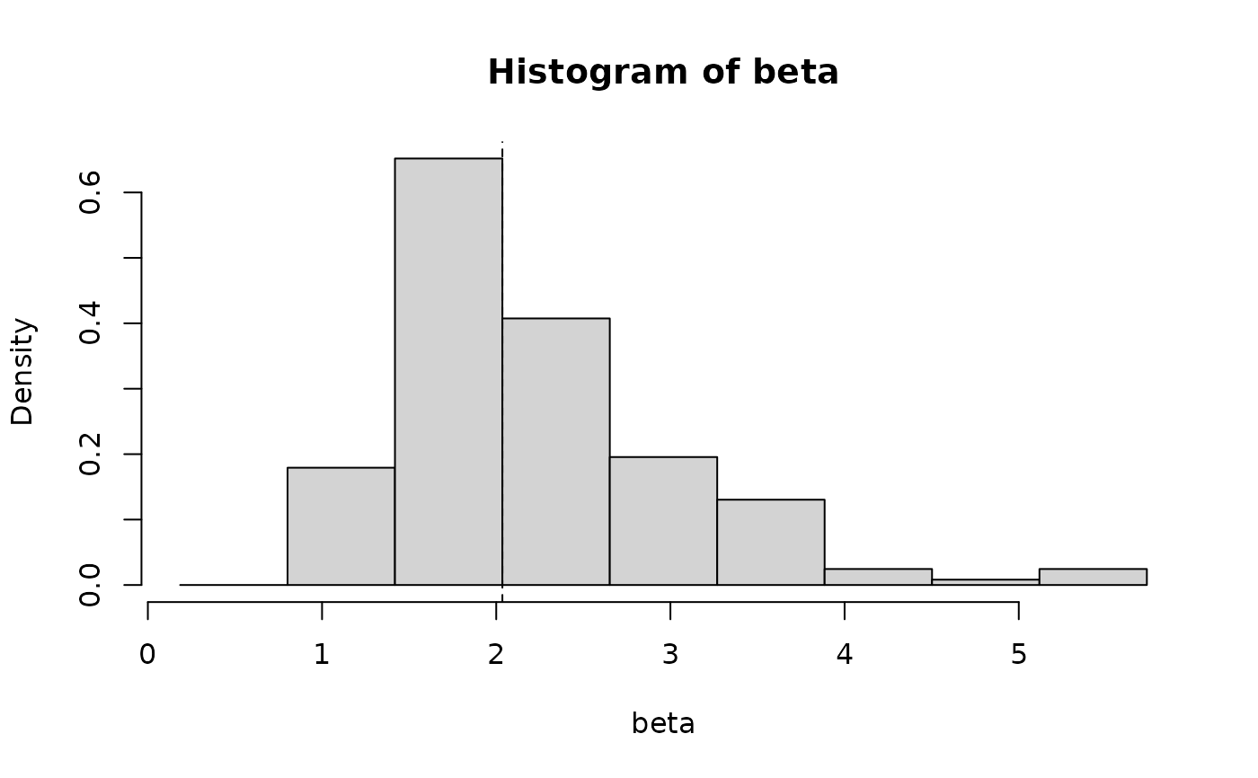
#Plot statistic distributions
plot(boot_est, index = "beta", type = "hist")