Subgroup Analysis After Propensity Score Matching Using R
matching
propensity-scores
R
subgroup analysis
Author
Noah Greifer
Published
September 5, 2022
Today I’m going to demonstrate performing a subgroup analysis after propensity score matching using R. Subgroup analysis, also known as moderation analysis or the analysis of effect modification, concerns the estimation of treatment effects within subgroups of a pre-treatment covariate. This post assumes you understand how to do propensity score matching. For a general introduction to propensity score matching, I recommend Austin (2011) and the MatchItintroductory vignette. If you understand inverse probability weighting but aren’t too familiar with matching, I recommend my article with Liz Stuart (Greifer and Stuart 2021). For an introduction to subgroup analysis with propensity scores, you can also check out Green and Stuart (2014). Here, I’ll mainly try to get to the point.
The dataset we’ll use today is the famous Lalonde dataset, investigating the effect of a job training program on earnings. We’ll use the version of this dataset that comes with the MatchIt package.
data("lalonde", package ="MatchIt")head(lalonde)
     treat age educ   race married nodegree re74 re75       re78
NSW1     1  37   11  black       1        1    0    0  9930.0460
NSW2     1  22    9 hispan       0        1    0    0  3595.8940
NSW3     1  30   12  black       0        0    0    0 24909.4500
NSW4     1  27   11  black       0        1    0    0  7506.1460
NSW5     1  33    8  black       0        1    0    0   289.7899
NSW6     1  22    9  black       0        1    0    0  4056.4940
The treatment is treat, the outcome in the original study was re78 (1978 earnings), and the other variables are pretreatment covariates that we want to adjust for using propensity score matching. In this example, I’ll actually be using a different outcome, re78_0, which is whether the participant’s 1978 earnings were equal to 0 or not, because I want to demonstrate the procedure for a binary outcome. So, we hope the treatment effect is negative, i.e., the risk of 0 earnings decreases for those in the treatment.
lalonde$re78_0 <-as.numeric(lalonde$re78 ==0)
Our moderator will be race, a 3-category factor variable.
with(lalonde, table(race))
race
 black hispan  white
   243     72    299
Our estimand will be the subgroup-specific and marginal average treatment effect on the treated (ATT), using the risk difference as our effect measure.
Packages You’ll Need
We’ll need a few R packages for this analysis. We’ll need MatchIt and optmatch for the matching, cobalt for the balance assessment, marginaleffects for estimating the treatment effects, and sandwich for computing the standard errors. You can install those using the code below:
Our first step is to perform the matching. Although there are a few strategies for performing matching for subgroup analysis, in general subgroup-specific matching tends to work best, though it requires a little extra work.
We’ll do this by splitting the dataset by race and performing a separate matching analysis within each one.
Here we’ll use full matching because 1:1 matching without replacement, the most common (but worst) way to do propensity score matching, doesn’t work well in this dataset. The process described below works exactly the same for 1:1 and most other kinds of matching as it does for full matching. We’ll estimate propensity scores in each subgroup, here using probit regression, which happens to yield better balance than logistic regression does.
library("MatchIt")#Matching in race == "black"m.out_b <-matchit(treat ~ age + educ + married + nodegree + re74 + re75,data = lalonde_b, method ="full", estimand ="ATT",link ="probit")#Matching in race == "hispan"m.out_h <-matchit(treat ~ age + educ + married + nodegree + re74 + re75,data = lalonde_h, method ="full", estimand ="ATT",link ="probit")#Matching in race == "black"m.out_w <-matchit(treat ~ age + educ + married + nodegree + re74 + re75,data = lalonde_w, method ="full", estimand ="ATT",link ="probit")
Step 2: Assessing Balance within Subgroups
We need to assess subgroup balance; we can do that using summary() on each matchit object, or we can use functions from cobalt.
Below are examples of using summary() and cobalt::bal.tab() on one matchit object at a time1:
summary(m.out_b)
Call:
matchit(formula = treat ~ age + educ + married + nodegree + re74 +
    re75, data = lalonde_b, method = "full", link = "probit",
    estimand = "ATT")

Summary of Balance for All Data:
         Means Treated Means Control Std. Mean Diff. Var. Ratio eCDF Mean eCDF Max
distance        0.6587        0.6121          0.4851     0.7278    0.1134   0.1972
age            25.9808       26.0690         -0.0121     0.4511    0.0902   0.2378
educ           10.3141       10.0920          0.1079     0.5436    0.0336   0.0807
married         0.1859        0.2874         -0.2608          .    0.1015   0.1015
nodegree        0.7244        0.6437          0.1806          .    0.0807   0.0807
re74         2155.0132     3117.0584         -0.1881     0.9436    0.0890   0.2863
re75         1490.7221     1834.4220         -0.1043     1.0667    0.0480   0.1441

Summary of Balance for Matched Data:
         Means Treated Means Control Std. Mean Diff. Var. Ratio eCDF Mean eCDF Max Std. Pair Dist.
distance        0.6587        0.6577          0.0099     1.0402    0.0096   0.0705          0.0376
age            25.9808       27.4679         -0.2037     0.3773    0.1105   0.2073          1.3627
educ           10.3141       10.1880          0.0612     0.6793    0.0199   0.0620          1.0428
married         0.1859        0.1822          0.0096          .    0.0037   0.0037          0.6540
nodegree        0.7244        0.7222          0.0048          .    0.0021   0.0021          0.7681
re74         2155.0132     2998.7354         -0.1650     0.7592    0.0513   0.2025          0.7291
re75         1490.7221     2130.0707         -0.1939     0.8840    0.0819   0.1976          0.8231

Sample Sizes:
              Control Treated
All             87.       156
Matched (ESS)   36.25     156
Matched         87.       156
Unmatched        0.         0
Discarded        0.         0
library("cobalt")bal.tab(m.out_b, un =TRUE, stats =c("m", "ks"))
Using the cluster argument produces balance tables in each subgroup and, because we specified cluster.summary = TRUE, a balance table summarizing across subgroups. To suppress display of the subgroup-specific balance tables (which may be useful if you have many subgroups), you can specify which.cluster = .none.
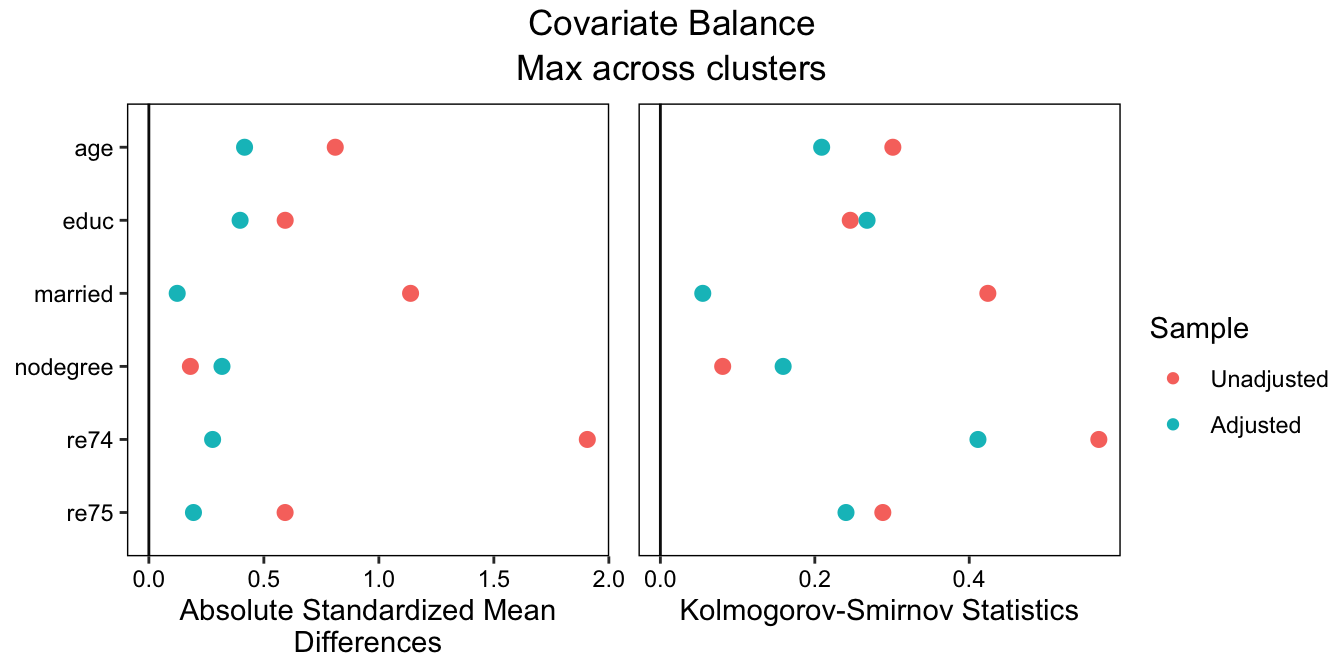
To make a plot displaying the balance statistics visually, we can use cobalt::love.plot():
From this output, we can see that balance is actually pretty bad; the greatest standardized mean difference (SMD) across subgroups after matching is around .46, which is way too big. In a realistic scenario, we would try different matching methods, maybe resorting to weighting, until we found good balance across the subgroups. In order to validly interpret the subgroup-specific effects and tests for moderation, we need to achieve balance in each subgroup, not just overall. We didn’t get good balance here, but to stay focused on the rest of the procedure, we’ll move forward as if we did.
Step 3: Fitting the Outcome Model
Next, we’ll fit the outcome model. It’s important to remember that the outcome model is an intermediate step for estimating the treatment effect; no quantity estimated by the model needs to correspond to the treatment effect directly. We’ll be using a marginal effects procedure to estimate the treatment effects in the next section.
First, we’ll extract the matched datasets from the matchit objects. We can’t just use the matching weights we extracted earlier because we also need subclass (i.e., pair) membership. We’ll use match_data() from MatchIt to extract the matched datasets, which contain the matching weights and subclass membership in the weights and subclass columns, respectively, and use rbind() to bind them into a single combined dataset2.
#Extract the matched datasetsmatched_data_b <-match_data(m.out_b)matched_data_h <-match_data(m.out_h)matched_data_w <-match_data(m.out_w)#Combine them using rbind()matched_data <-rbind(matched_data_b, matched_data_h, matched_data_w)names(matched_data)
Next, we can fit the outcome model. The choice of which model to fit should depend primarily on the best model for the outcome; because we have a binary outcome, we’ll use logistic regression.
It’s usually a good idea to include covariates in the outcome model. It’s also usually a good idea to allow the treatment to interact with the covariates in the outcome model. It’s also usually a good idea to fit separate models within each subgroup. Combining this all yields a pretty complicated model, which is why it will be so important to use a marginal effects procedure rather than trying to interpret the model’s coefficients. Here’s how we fit this model:
We’re not even going to look at the output of this model, which has 42 parameters. If the model doesn’t fit with your dataset, you can remove interactions between the treatment and some covariates or remove the covariates altogether.
For a linear model, you can use lm() and remove the family argument. We used family = "quasibinomial" because we want logistic regression for our binary outcome but we are using the matching weights, which otherwise create a (harmless but annoying) warning when run with family = "binomial".
Step 4: Estimate the Treatment Effects
Finally, we can estimate the treatment effects. To do so, we’ll use an average marginal effects procedure as implemented in marginaleffects. First, we’ll estimate the average marginal effect overall, averaging across the subgroups. Again, we’re hoping for a negative treatment effect, which indicates the risk of having zero income decreased among those who received the treatment. Because we are estimating the ATT, we need to subset the data for which the average marginal effects are computed to just the treated units, which we do using the newdata argument (which can be omitted when the ATE is the target estimand). We also need to supply pair membership to ensure the standard errors are correctly computed, which we do by supplying the subclass variable containing pair membership to the vcov argument.
library("marginaleffects")#Estimate the overall ATTavg_comparisons(fit, variables ="treat",newdata =subset(treat ==1),vcov =~subclass)
The estimated risk difference is 0.0305 with a high p-value and a confidence interval containing 0, indicating no evidence of an effect overall. (Note: this doesn’t mean there is no effect! The data are compatible with effects anywhere within the confidence interval, which includes negative and positive effects of a moderate size!)
New, let’s estimate the subgroup-specific effects by supplying the subgrouping variable, "race", to the by argument:
Here, we see that actually there is evidence of treatment effects within subgroups! In the subgroups hispan and white, we see moderately sized negative effects with small p-values and confidence intervals excluding 0, suggesting that there treatment effects in these subgroups.
We can also test whether the treatment effects differ between groups using the hypothesis argument of avg_comparisons():
We can see evidence that the treatment effect differs between the black and hispan groups, and between the black and white groups. With many subgroups, it might be useful to adjust your p-values for multiple comparisons, which we can do by supplying an argument to p_adjust.
If you want a single omnibus test for the presence of moderation, you can supply the output of the above to hyppotheses() with joint = TRUE, which we do below3. Note that because one of the comparisons is redundant, we need to change hypothesis to ~reference in the call to avg_comparisons().
A fair bit needs to be included when reporting your results to ensure your analysis is replicable and can be correctly interpreted by your audience. The key things to report are the following:
The method of estimating the propensity score and performing the matching (noting that these were done within subgroups), including the estimand targeted and whether that estimand was respected by the procedure (using, e.g., a caliper changes the estimand from the one you specify). This should also include the packages used and, even better, the functions used. If you’re using MatchIt, the documentation should also tell you which papers to cite.
A quick summary of other methods you might have tried and why you went with the one you went with (i.e., because it yielded better balance, a greater effective sample size, etc.).
Covariate balance, measured broadly; this can include a balance table, a balance plot (like one produced by cobalt::love.plot()), or a summary of balance (like providing the largest SMD and KS statistic observed across subgroups). Make sure your description of balance reflects the subgroups, e.g., by having separate tables or plots for each subgroup or clarifying that the statistics presented are averages or the worst case across subgroups.
The outcome model you used, especially specifying the form of the model used and how/whether covariates entered the model. Also mention the method used to compute the standard errors (e.g., cluster-robust standard errors with pair membership as the clustering variable).
Details of the marginal effects procedure used, including the package used, and the method to compute the standard errors (in this case, the delta method, which is the only method available in marginaleffects).
The treatment effect estimates along with their p-values and confidence intervals, both overall, within subgroups, and for the omnibus test.
References
Austin, Peter C. 2011. “An Introduction to Propensity Score Methods for Reducing the Effects of Confounding in Observational Studies.”Multivariate Behavioral Research 46 (3): 399–424. https://doi.org/10.1080/00273171.2011.568786.
Green, Kerry M., and Elizabeth A. Stuart. 2014. “Examining Moderation Analyses in Propensity Score Methods: Application to Depression and Substance Use.”Journal of Consulting and Clinical Psychology, Advances in Data Analytic Methods, vol. 82 (5): 773–83. https://doi.org/10.1037/a0036515.
Greifer, Noah, and Elizabeth A Stuart. 2021. “Matching Methods for Confounder Adjustment: An Addition to the Epidemiologist’s Toolbox.”Epidemiologic Reviews, June, mxab003. https://doi.org/10.1093/epirev/mxab003.
Footnotes
You might notices the mean differences for binary variables differ between the two outputs; that’s because summary() standardizes the mean differences whereas bal.tab() does not for binary variables. If you want standardized mean differences for binary variables from bal.tab(), just add the argument binary = "std".↩︎
Note: rbind() must be used for this; functions from other packages, like dplyr::bind_rows(), will not correctly preserve the subclass structure.↩︎
We also set joint_test = "chisq" to use a \(\chi^2\) test, which is more appropriate for binary outcomes.↩︎